
Facebook’s web tier is one of the main services that handle HTTP requests from people using our services each time they interact with Facebook. It is a massive global service distributed across multiple data centers throughout the world. Since we have people from all over the world using our services, the load on the web tier varies throughout the day, depending on the number of people using our service at any given time. To manage the load on our services, we use throughput autoscaling. Throughput autoscaling is designed to estimate a service’s capacity requirements based on the amount of work that the service needs to perform at a given time.
Our peak load generally happens when it’s evening in Europe and Asia and most of the Americas are also awake. From there, the load slowly decreases, reaching its lowest point in the evening, Pacific Time. Since our global load balancer, Taiji, works to maintain a similar load level across all our data center regions, they all experience the same peak and off-peak pattern. The web tier needs to have enough global capacity to handle the peak load — without leaving machines sitting underutilized during off-peak times. We need an additional disaster recovery buffer (DR buffer) to be prepared for any disaster that might cause the largest data center region to become unavailable. We also need to account for engagement growth, new feature launches, and other operational buffers.
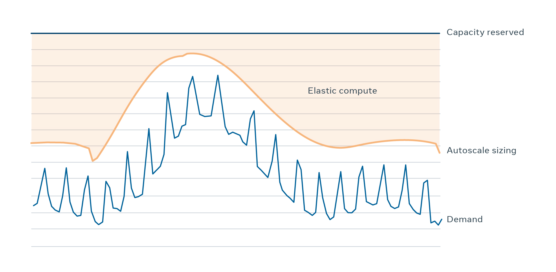
Before autoscale, we statically sized the web tier, which means that we manually calculated the amount of global capacity we needed to handle the peak load with the DR buffer for a certain projected period of time. That capacity was then allocated and dedicated exclusively to the web tier at all times. Since adding capacity was a manual process, we also kept a higher percentage of extra safety buffers.
This was very inefficient, as the web tier didn’t need all those machines at all hours. It needed all of them for a couple of hours around our traffic peak for the final few weeks of a capacity planning cycle. After we applied autoscale, we could dynamically size the web tier closer to its needs through the day. Outside of peak hours, autoscale gradually removes and then adds back a considerable amount of capacity while keeping individual machines running with loads similar to what they run at peak times. Since the web tier is massive and the difference between peak and off-peak demand is large, application of autoscaling frees a considerable number of machines, which are then used for running other workloads, such as machine learning (ML) models.
While improved utilization of computing resources is the main motivation behind applying autoscaling to the web tier, we needed to do so while maintaining safety. Therefore, the accuracy of throughput autoscaling is critical to enable this goal. Throughput autoscaling allows us to model sufficient capacity to a high degree of accuracy, which enables us to use our resources more efficiently than other modeling techniques would. We have been successfully applying the throughput modeling methodology to autoscale the web tier for the past two years.
Throughput autoscaling: Workload-driven sizing
Throughput autoscaling makes sizing decisions based on the amount of work that the service needs to perform as measured by throughput metrics. The definition of throughput is a measure of the useful work performed by a service in absolute terms. For example, requests per second (RPS), also referred to as queries per second (QPS), is one of the most common throughput metrics. Another example is the number of elements ranked per second for an ML service that ranks elements to prioritize which to display to a person using the site. Since the useful work for a request varies for ML services, the number of ranked elements capture throughput better than RPS does. These throughput metrics differ from utilization metrics, which are more commonly used in the industry for autoscaling. The key difference between throughput and utilization metrics is that throughput is an absolute metric of work performed and is not impacted by the number of servers performing that work. As utilization is a normalized measure of system load, distributing that load among more or fewer servers will impact utilization. Throughput autoscaling estimates current supply and disaster demand in terms of a throughput metric:
- Current supply: Total throughput that a service can handle using the current capacity provision for that service at a given data center region.
- Disaster demand: Total throughput required of a service in a given data center region when serving additional demand due to the loss of computational resources in another data center region.
Throughput autoscaling calculates the number of hosts to which a service should be deployed by comparing current supply and disaster demand. If the anticipated disaster demand is higher than the current supply, autoscale increases the capacity so that the service is prepared to handle the disaster demand. Conversely, when current supply is too high, autoscale will decrease the capacity so that the service runs more efficiently. This allows throughput autoscaling to model the number of machines required for a given workload, even when that workload has not yet been observed historically. This is one of the key benefits of a throughput-based approach over a utilization-based one.
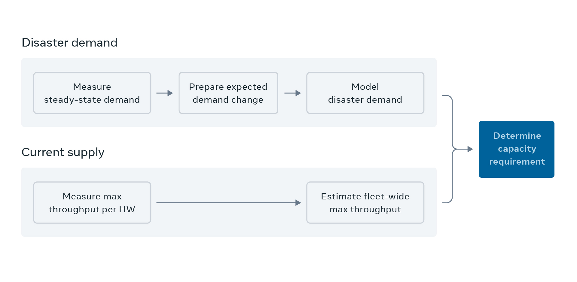
Predicting disaster demand
Let’s take a look at the details of each step:
- Model predicted steady-state demand
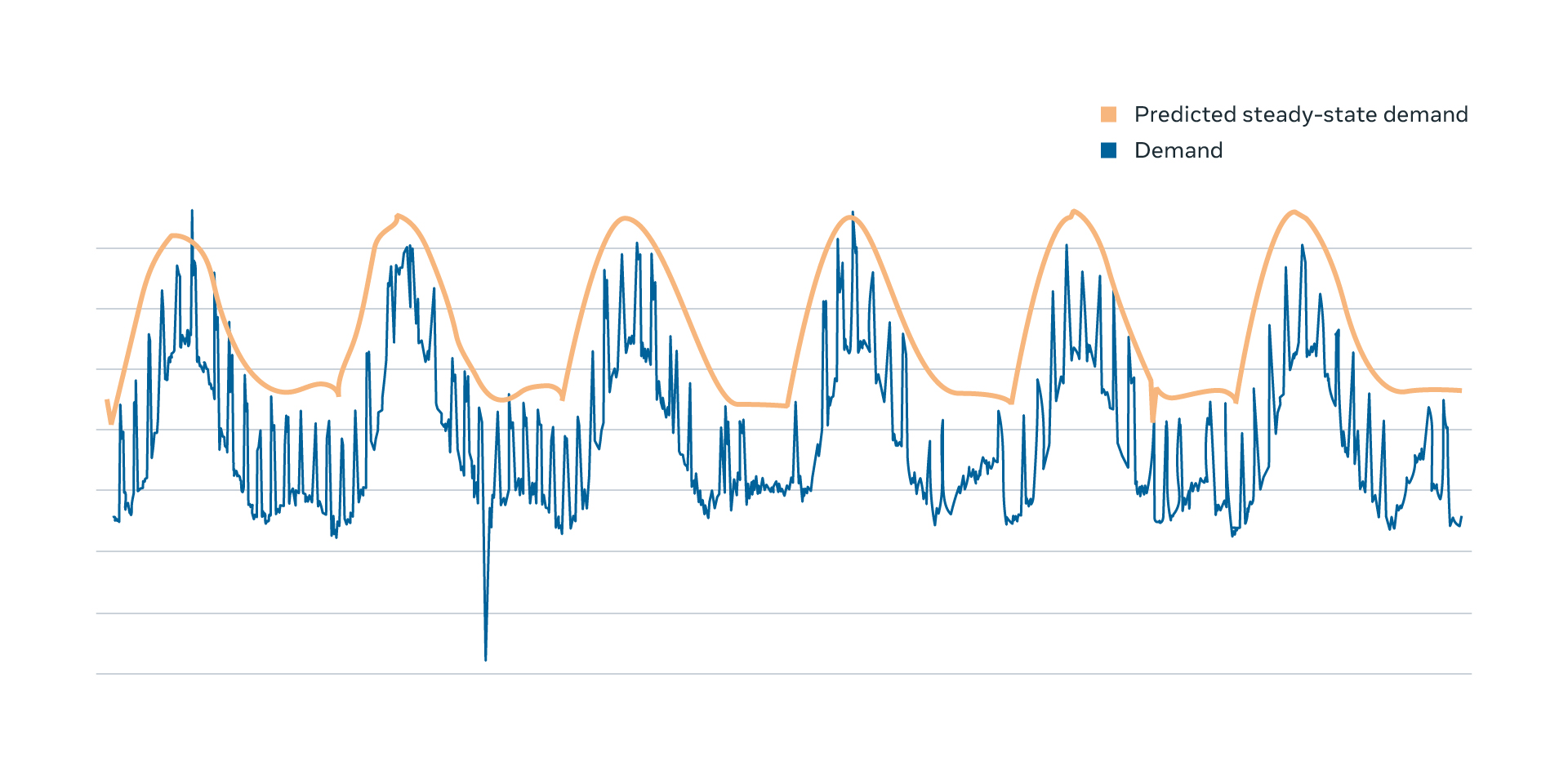
To estimate disaster demand, we start by measuring the actual steady-state demand. A throughput metric, such as QPS, is measured at the individual server and then aggregated into a data-center granularity (i.e., regional demand). These measurements of historical demand are used to train ML models to discern patterns in their seasonality. Then, during capacity modeling, we predict future steady-state demand by querying these ML models. The output of the models are compared with live measurements to ensure that the service’s behavior has not deviated from historical patterns.
Using predicted demand is beneficial in that it increases safety by upsizing in advance, taking probable future demand increase into account. It is particularly useful for services that require a long startup/shutdown time. Predicted demand also improves the stability of autoscaling by removing high order terms from these predictions. For example, a new binary push for the web tier creates periods of elevated workload for warmup. Frequent capacity changes between pushes would add unnecessary capacity fluctuation.
Next, we apply a set of expected demand changes. The observed demand in a given data center region is often expected to change. For example, a feature launch from a client service or a holiday may have a significant impact on demand. A maintenance event in infrastructure can also affect the service’s demand, e.g., the traffic at a data center region will change when new hardware is brought online or old hardware is decommissioned.
- Model disaster demand
Another important aspect of capacity requirements for Facebook services is disaster readiness. Disasters come in a variety of forms, including networking equipment outages, and regional weather events, such as hurricanes. These can occur with limited notice and, in worst-case scenarios, can make an entire data center region’s resources unavailable for some period of time. When a data center region becomes unavailable, our infrastructure responds by redistributing user traffic to the others. To ensure that we continue to serve the people using our services in a disaster situation, we need to size our services with this redistribution in mind. This means that in addition to the steady-state demand, we also need to consider the extra demand each data center region will receive in the worst-case scenario — when the largest data center region is down. We call this the disaster demand.
To estimate the disaster demand, throughput autoscaling simulates the loss of the largest data center region and calculates how much extra demand would be distributed to each of the other data center regions. It uses the fact that Taiji redistributes the lost data center region’s traffic to the remaining regions, proportional to the size of each region In other words, a large data center region will get more extra traffic than a small data center region at the time of disaster. It then sums up this extra disaster demand with the predicted steady-state demand and outputs a predicted disaster demand that is used to calculate the optimal size of the service.
Estimating supply through load testing
Understanding the disaster demand does us little good without knowing whether the currently provisioned containers would be able to withstand the disaster workload demanded of them. The current deployment will be able to handle some maximum throughput before degrading to unacceptable levels of performance, such as an unacceptably high error rate or latency. We refer to this maximum throughput as the throughput supply. The goal of autoscaling is to adjust the number of containers that a service is deployed to such that supply will be as close to the disaster demand as feasible without dropping below it.
In order to measure throughput supply, we need to understand the contribution of each machine to which the service is deployed. We accomplish this by leveraging our internal load testing platform. These load tests move increasing amounts of production traffic to a small number of target hosts. The movement of production traffic allows us to understand the actual response to organic increases in demand that may be missed through the use of simulated traffic. These load tests monitor the target hosts and back off once the hosts reach a degraded state. We can use data from the load test to measure throughput for periods of time where service metrics are just below degraded. In this way, we can map individual hosts to their maximum safe throughput.
These load tests take place throughout the day, every day, to provide constant monitoring of increases and decreases in the supplied throughput per host. They also target each region and hardware profile that a service utilizes to understand how a host’s regionality and hardware affect its throughput. Once the throughput per region and hardware profile are understood, we can aggregate these per-machine measurements into an estimate of the full regional supply at a given point in time. Then, if this supply is too small or large for the predicted disaster demand, we can use this load test data to estimate the number of machines we should add or remove.
Putting it all together
As an example, let’s examine a theoretical service, which is deployed to three distinct regions that we’ll call U.S. West, U.S. East, and Europe. The following table shows the result of each step described below:
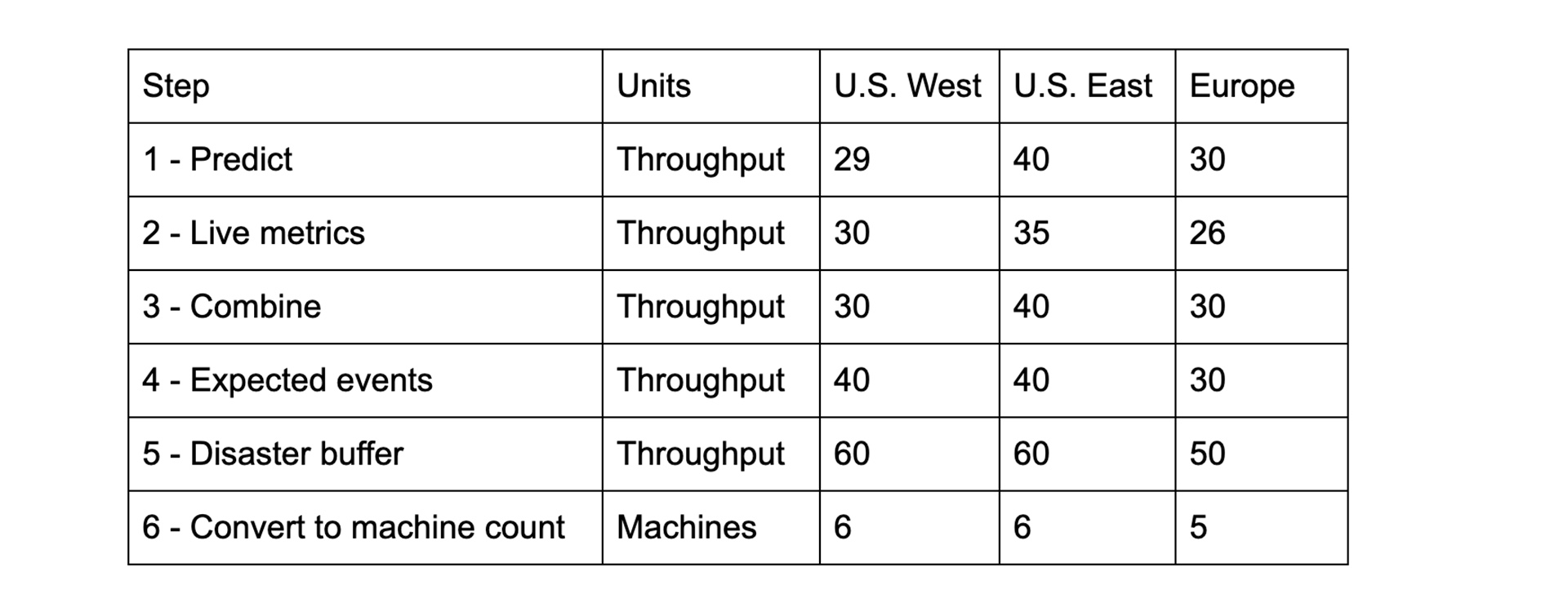
- Query the ML models for predictions of demand expected in the next hour.
- Query the live state for the service. In this example, all regions are experiencing demand that is less than the output of our predictive model except for the U.S. West region.
- Aggregate the predictions with the measurements. As we optimize for safety, we will aggregate using the maximum to err on the side of caution. This means that we’ll use the predicted number in all regions except for U.S. West, where we will use the live metrics.
- Let’s assume that we have an imminent infrastructure change that is expected to affect this service within the period we are sizing for. In this example, we will be shifting some of the front-end traffic that affects this service in such a way that 25 percent of U.S. East demand will go to U.S. West. This will increase the anticipated demand in U.S. West. However, as the demand has not yet moved, we still need to handle the current demands in U.S. East. So, we will modify only U.S. West.
- As we mentioned earlier, disaster readiness requires us to expect that the worst-case scenario region will be down. For simplicity, let’s assume each region redistributes equally to the remaining regions. This means that U.S. West going down is the worst possible scenario for U.S. East and Europe demand, since it would increase demand by 20 units each. For U.S. West, U.S. East going down would result in 20 units of increased demand. Therefore, all regions need to have a disaster buffer equal to 20 units of throughput.
- The final step is to turn this demand into a machine count. Let’s assume we can handle 10 units of demand per machine based on our recent load tests. Then, we are able to compute a final size through simple division.
A keen observer will note that this example glosses over many of the details covered above, including load balancer behavior, the impact of regionality and hardware specifications on throughput supply, etc. Handling these issues is important for acceptable operation of the model, but we’ve skipped them here, as they complicate the example and would be tied to implementation details specific to each company.
Capacity model validation
Like any model, our capacity model will have some level of error. The concept of throughput metrics, which are intended to measure the useful work performed by a service, is an important component of our capacity model. As such, the unit for this metric must uniformly measure work in order for the metric to have high quality. Consider queries per second (QPS). Would it make a quality throughput metric? After all, queries are the work that the service is operating on. More queries means more work. However, for the majority of services, an individual query may represent a different amount of work. The web tier readily represents a counterexample, as the work requirements will vary remarkably between retrieving the News Feed versus a deep link to a specific post. Therefore, using QPS as the throughput metric for the web tier could result in high errors should they not be uniformly distributed across our infrastructure. A redistribution of cheaper requests would require fewer machines than we would expect, and a redistribution of more expensive requests would require more.
Errors as a result of throughput metric quality will manifest in the measurement of the supply of throughput available, the measurement of historical and current throughput demands, and the prediction of future demands. Supply may have some level of error due to the load testing methodology applied, demand may have errors from the ML models, and our simulation of load balancer responses to various scenarios may introduce other errors. In the presence of these myriad potential sources of error, how do we build confidence in our model? We measure and validate the accuracy of the system.
Where possible, we want to validate the individual steps in the capacity modeling process. This allows us to understand where investment in improvements would have the greatest impact and alleviates concerns of offsetting errors. Getting the correct final result by accident is not particularly useful if these offsetting errors are not guaranteed in future operations. An example of such a validation is the evaluation of our steady-state demand predictions. These ML models produce predictions of demand under normal conditions at specified times of day. We can compare these predictions with actual demand during time periods considered to be normal. As these predictions are expected to be greater than actuals, we focus mostly on periods of time where we have underestimated the actual demands.
To ensure that the entire system works in a sufficiently safe manner, we also need to validate the whole system end to end. However, as the system is quite complex, it is often necessary to validate in terms of specific scenarios. To validate the disaster readiness component of our estimates, we are able to leverage disaster drills. These company-wide exercises simulate a disaster by disconnecting a data center region from the production network, and they provide a valuable opportunity to observe the behavior of the system in disaster-like situations. We can compare our capacity models prior to the disaster with measurements of the observed behavior to understand our level of error. Similar comparisons are possible for other scenarios, such as hardware turn-ups and decommissions.
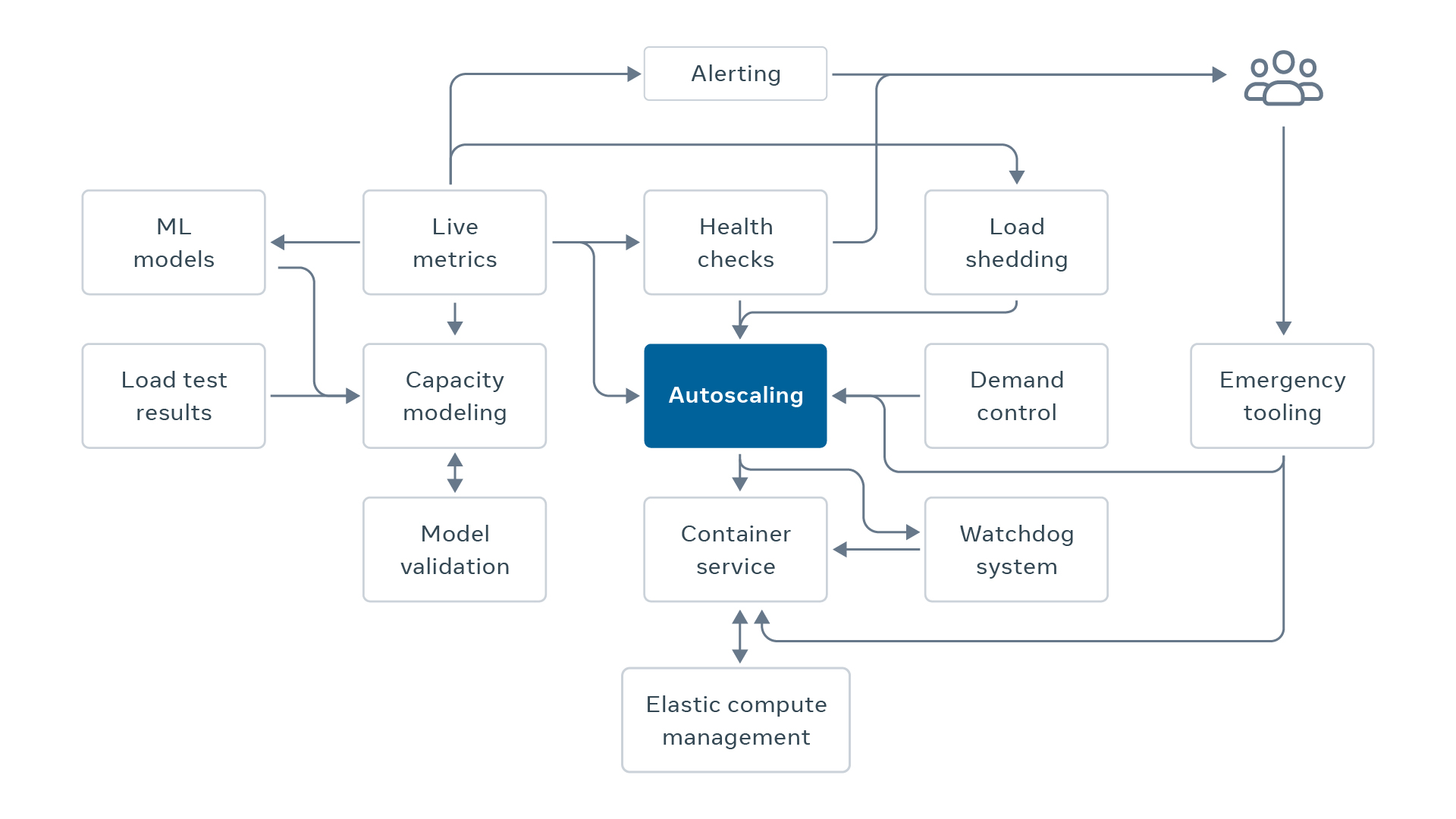
The service capacity management ecosystem
The throughput autoscaling capacity model allows us to understand the correct capacity for a service. However, this understanding is only one piece of the autoscaling puzzle. We need an end-to-end autoscaling system that takes this size and mutates the number of containers running the service in a safe, reliable, and predictable manner. This mutation needs to be performed in a controlled way to ensure continued service health. As humans are less and less involved in day-to-day sizing, automation failures must be detected and handled accordingly. Finally, this freed capacity must be made available to other workloads in order to realize the full benefits of autoscaling.
Safety mechanisms
While dynamic sizing is undoubtedly more efficient, especially for services like our web tier that have a diurnal load pattern, it also introduces the risk of depending on the autoscale automation to quickly and correctly size the service.
There are multiple scenarios that could cause problems:
- The demand could increase above the disaster demand predicted by the modeling, because of either unexpected demand surge or prediction error.
- The autoscale automation could have an outage and not upsize the service when approaching peak.
- The autoscale automation could misbehave and downscale the service too much when going off peak.
In order to address these risks, we have introduced a series of safety mechanisms. They mitigate these risks and help ensure that we are not affecting the reliability of the service by dynamically sizing it.
Reactive algorithm in throughput autoscaling
We always use the predictive autoscaling algorithm, which uses the predicted disaster demand explained above, together with a reactive autoscaling algorithm. The reactive autoscaling algorithm looks at the current demand, which is the total throughput that the service is serving at a given point in time. The algorithm adds a small percentage of extra buffer and uses that to calculate desirable capacity size.
Throughput autoscaling chooses whichever is larger, predictive size or reactive size. In normal operation, the reactive size is smaller than the predictive size. However, reactive size can be dominant if a service experiences an unexpected increase in demand that is a lot larger than the previous days’ demand. Predictive sizing is preferred for normal situations that respect the same daily pattern, as it can upsize the service in advance of experiencing increased demand. Reactive is mostly used as a failsafe mechanism in a situation when current demand gets too close to current supply.
Watchdog
As the name suggests, a watchdog is an auxiliary service that monitors the success of autoscale automation by periodically checking the heartbeat from autoscaling. If the heartbeat is not updated for more than a certain configured time, it will bring the service’s capacity back to a safe size, which in most cases is the max of the last seven days. This ensures the safety of autoscaling by bringing the service’’s capacity back when an unexpected failure happens in the critical path (and downstream dependencies).
Since this is a last defense to prevent catastrophic failure, it was important that we keep this service very simple, with minimal dependencies. Also, since breakages in autoscale automation could be due to new binary release, it is important not to reuse code between the two.
Prevent inaccurate sizing and sizing verification
The autoscale system uses a variety of data sources to make an accurate estimation from the load testing data to the current mixture of hardware of a service. We have a stage to validate the quality of input data and return a confidence level of the capacity estimation. For example, if the maximum throughput measured by the load testing is not stable, or if there are not enough data points, the confidence level will drop. Autoscaling will then stop operating and the watchdog will kick in, bringing the capacity back to the safe level.
Throughout the resizing, autoscale performs a set of safety checks to validate success of sizing, such as completion of resize, within a desirable time window, service health (to ensure a service doesn’t become unhealthy during downsize), status of cross-region traffic (to avoid downsizing services that are shedding load), overall service size (to prevent downsizing in deficit), and so on. If anything looks awry, autoscale will revert to the original size.
Small-step size
Another safety mechanism is downsizing in small steps. Large steps can take a service from healthy to very unhealthy. Small steps allow early signs of problems to stop the process. Each service can configure the maximum change in size, expressed as percent of total service capacity, over a time window. For example, a service could configure a downsize limit of 5 percent over a 15-minute window. By making smaller changes over more time, we allow detection mechanisms, like alerting and health checks, to observe whether the service might be becoming undersized with plenty of time to react before it reaches a critical state.
Autoscaling the Facebook web tier
By using the autoscale methodology and having all these safety mechanisms, we have been dynamically sizing the Facebook web tier for more than a year now. This allows us to free up servers reserved for web at off-peak time and let other workloads to run until web needs them back for the peak time. The number of servers we can repurpose is considerably large because web is a large service with a significant difference between peak and trough.
All unneeded servers go into the elastic compute pool at Facebook. This pool contains the servers that are not currently being used by the original workloads. It’s called elastic because its size varies, and machines can come in and go out at any time.
We have a large number of workloads that leverage the elastic compute pool. They usually are short-lived and latency-insensitive jobs that can be run asynchronously, such as time shifting async jobs or ML model training jobs. For example, we use those servers for generating better feed ranking or better ads, or for detecting and preventing harmful content from appearing on our platform. Instead of needing extra capacity, we can now use those servers that sat underutilized in the web tier before.
Conclusion
The autoscaling methodology in Facebook enables us to correctly and safely size our services without compromising reliability. After we proved its functionality using web tier for a year, we started to apply it to other large services, such as Django web service for Instagram and multifeed services. We are in the process of deploying autoscaling to a broader set of Facebook web and Instagram back-end services that show a diurnal demand pattern. As more servers are released into the elastic compute pool, we will have a bigger opportunity to identify workloads that can move from having dedicated capacity available to them all the time to running on the elastic compute pool.
Through autoscale and elastic compute, we can use our hardware more efficiently to keep up with our increasing computing demands for the new products on Facebook, Instagram, and WhatsApp. We will be able to support more people using our products and more services running critical ML workloads.
We will be hosting a talk about our work on throughput autoscaling through optimal workload placement during our virtual Systems @Scale event at 11am PT on Wednesday, September 16, followed by a live Q&A session. Please submit any questions you may have to systemsatscale@fb.com before the event.


")


