
- Explore is one of the largest recommendation systems on Instagram.
- We leverage machine learning to make sure people are always seeing content that is the most interesting and relevant to them.
- Using more advanced machine learning models, like Two Towers neural networks, we’ve been able to make the Explore recommendation system even more scalable and flexible.
AI plays an important role in what people see on Meta’s platforms. Every day, hundreds of millions of people visit Explore on Instagram to discover something new, making it one of the largest recommendation surfaces on Instagram.
To build a large-scale system capable of recommending the most relevant content to people in real time out of billions of available options, we’ve leveraged machine learning (ML) to introduce task specific domain-specific language (DSL) and a multi-stage approach to ranking.
As the system has continued to evolve, we’ve expanded our multi-stage ranking approach with several well-defined stages, each focusing on different objectives and algorithms.
- Retrieval
- First-stage ranking
- Second-stage ranking
- Final reranking
By leveraging caching and pre-computation with highly-customizable modeling techniques, like a Two Towers neural network (NN), we’ve built a ranking system for Explore that is even more flexible and scalable than ever before.
Readers might notice that the leitmotif of this post will be clever use of caching and pre-computation in different ranking stages. This allows us to use heavier models in every stage of ranking, learn behavior from data, and rely less on heuristics.
Retrieval
The basic idea behind retrieval is to get an approximation of what content (candidates) will be ranked high at later stages in the process if all of the content is drawn from a general media distribution.
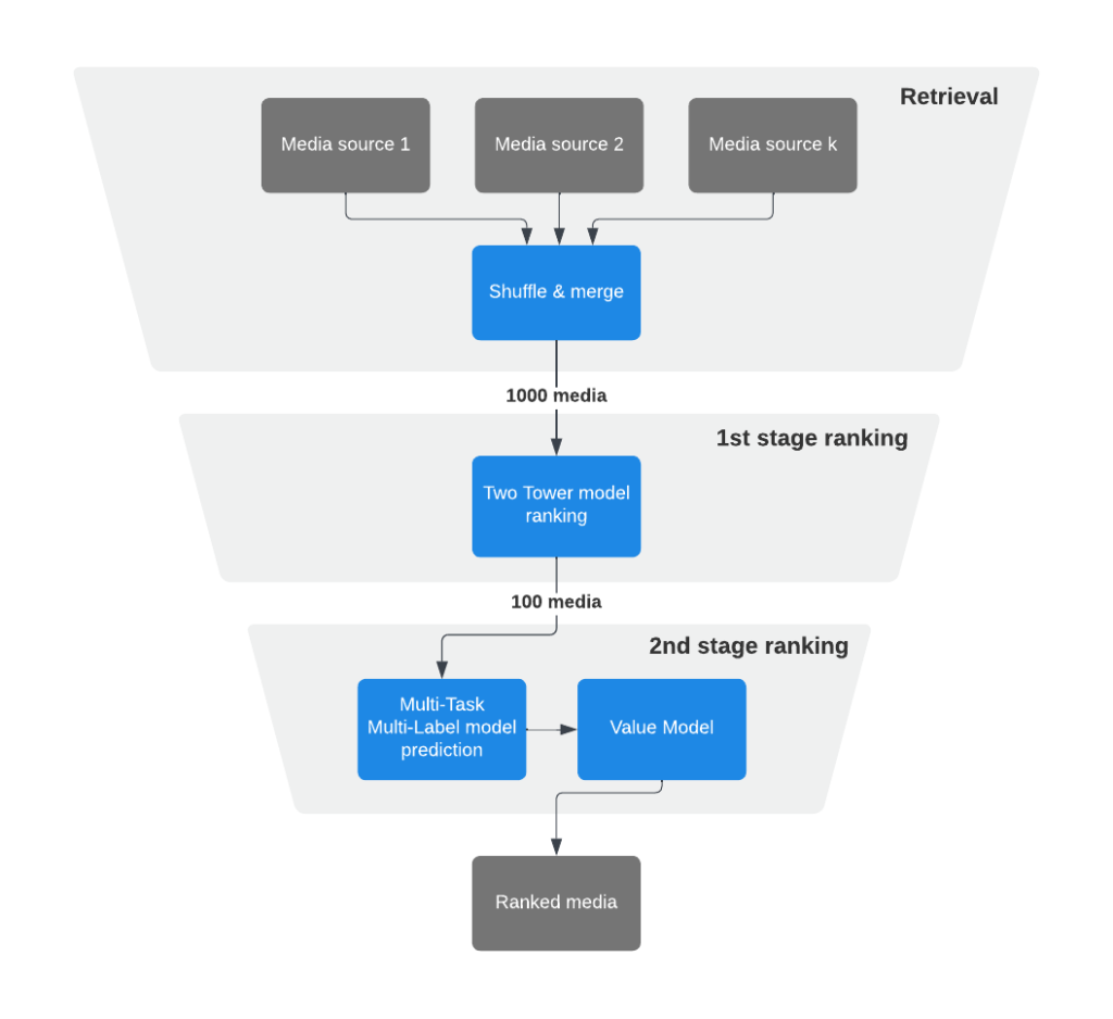
In a world with infinite computational power and no latency requirements we could rank all possible content. But, given real-world requirements and constraints, most large-scale recommender systems employ a multi-stage funnel approach – starting with thousands of candidates and narrowing down the number of candidates to hundreds as we go down the funnel.
In most large-scale recommender systems, the retrieval stage consists of multiple candidates’ retrieval sources (“sources” for short). The main purpose of a source is to select hundreds of relevant items from a media pool of billions of items. Once we fetch candidates from different sources, we combine them together and pass them to ranking models.
Candidates’ sources can be based on heuristics (e.g., trending posts) as well as more sophisticated ML approaches. Additionally, retrieval sources can be real-time (capturing most recent interactions) and pre-generated (capturing long-term interests).
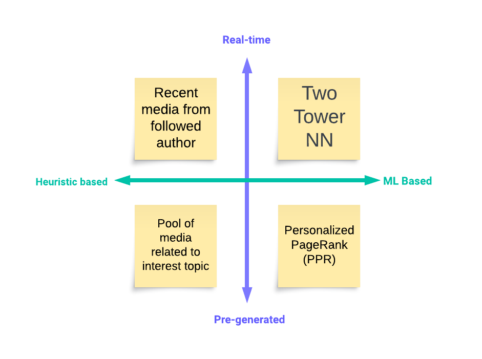
To model media retrieval for different user groups with various interests, we utilize all these mentioned source types together and mix them with tunable weights.
Candidates from pre-generated sources could be generated offline during off-peak hours (e.g., locally popular media), which further contributes to system scalability.
Let’s take a closer look at a couple of techniques that can be used in retrieval.
Two Tower NN
Two Tower NNs deserve special attention in the context of retrieval.
Our ML-based approach to retrieval used the Word2Vec algorithm to generate user and media/author embeddings based on their IDs.
The Two Towers model extends the Word2Vec algorithm, allowing us to use arbitrary user or media/author features and learn from multiple tasks at the same time for multi-objective retrieval. This new model retains the maintainability and real-time nature of Word2Vec, which makes it a great choice for a candidate sourcing algorithm.
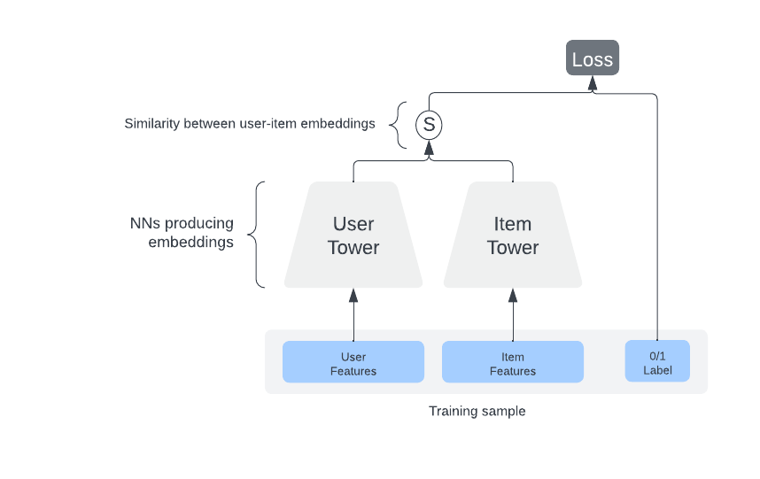
Here’s how the Two Tower retrieval works in general with schema:
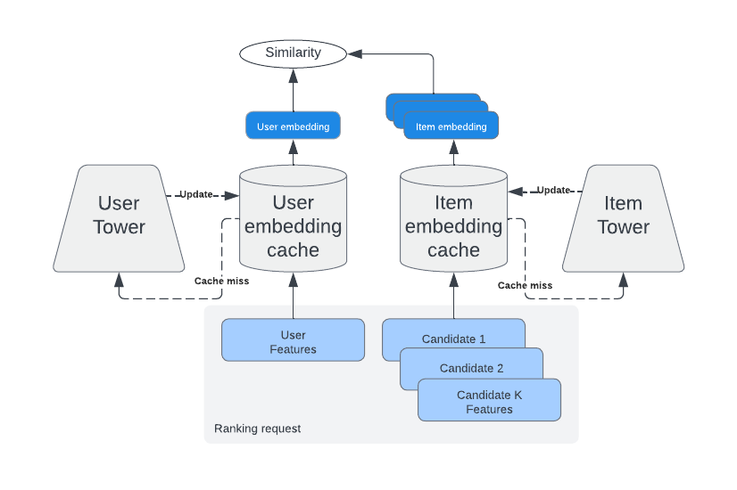
- The Two Tower model consists of two separate neural networks – one for the user and one for the item.
- Each neural network only consumes features related to their entity and outputs an embedding.
- The learning objective is to predict engagement events (e.g., someone liking a post) as a similarity measure between user and item embeddings.
- After training, user embeddings should be close to the embeddings of relevant items for a given user. Therefore, item embeddings close to the user’s embedding can be used as candidates for ranking.
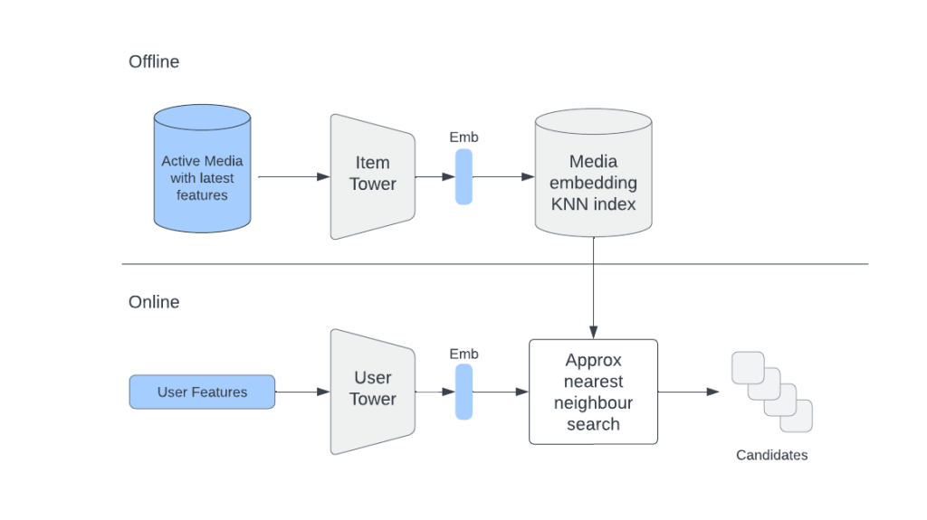
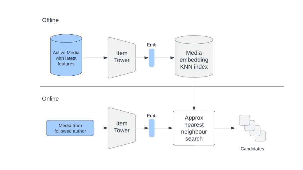
Given that user and item networks (towers) are independent after training, we can use an item tower to generate embeddings for items that can be used as candidates during retrieval. And we can do this on a daily basis using an offline pipeline.
We can also put generated item embeddings into a service that supports online approximate nearest neighbors (ANN) search (e.g., FAISS, HNSW, etc), to make sure that we don’t have to scan through an entire set of items to find similar items for a given user.
During online retrieval we use the user tower to generate user embedding on the fly by fetching the freshest user-side features, and use it to find the most similar items in the ANN service.
It’s important to keep in mind that the model can’t consume user-item interaction features (which are usually the most powerful) because by consuming them it will lose the ability to provide cacheable user/item embeddings.
The main advantage of the Two Tower approach is that user and item embeddings can be cached, making inference for the Two Tower model extremely efficient.
User interactions history
We can also use item embeddings directly to retrieve similar items to those from a user’s interactions history.
Let’s say that a user liked/saved/shared some items. Given that we have embeddings of those items, we can find a list of similar items to each of them and combine them into a single list.
This list will contain items reflective of the user’s previous and current interests.
Compared with retrieving candidates using user embedding, directly using a user’s interactions history allows us to have a better control over online tradeoff between different engagement types.
In order for this approach to produce high-quality candidates, it’s important to select good items from the user’s interactions history. (i.e., If we try to find similar items to some randomly clicked item we might risk flooding someone’s recommendations with irrelevant content).
To select good candidates, we apply a rule-based approach to filter-out poor-quality items (i.e., sexual/objectionable images, posts with high number of “reports”, etc.) from the interactions history. This allows us to retrieve much better candidates for further ranking stages.
Ranking
After candidates are retrieved, the system needs to rank them by value to the user.
Ranking in a high load system is usually divided into multiple stages that gradually reduce the number of candidates from a few thousand to few hundred that are finally presented to the user.
In Explore, because it’s infeasible to rank all candidates using heavy models, we use two stages:
- A first-stage ranker (i.e., lightweight model), which is less precise and less computationally intensive and can recall thousands of candidates.
- A second-stage ranker (i.e., heavy model), which is more precise and compute intensive and operates on the 100 best candidates from the first stage.
Using a two-stage approach allows us to rank more candidates while maintaining a high quality of final recommendations.
For both stages we choose to use neural networks because, in our use case, it’s important to be able to adapt to changing trends in users’ behavior very quickly. Neural networks allow us to do this by utilizing continual online training, meaning we can re-train (fine-tune) our models every hour as soon as we have new data. Also, a lot of important features are categorical in nature, and neural networks provide a natural way of handling categorical data by learning embeddings
First-stage ranking
In the first-stage ranking our old friend the Two Tower NN comes into play again because of its cacheability property.
Even though the model architecture could be similar to retrieval, the learning objective differs quite a bit: We train the first stage ranker to predict the output of the second stage with the label:
PSelect = { media in top K results ranked by the second stage}
We can view this approach as a way of distilling knowledge from a bigger second-stage model to a smaller (more light-weight) first-stage model.
Second-stage ranking
After the first stage we apply the second-stage ranker, which predicts the probability of different engagement events (click, like, etc.) using the multi-task multi label (MTML) neural network model.
The MTML model is much heavier than the Two Towers model. But it can also consume the most powerful user-item interaction features.
Applying a much heavier MTML model during peak hours could be tricky. That’s why we precompute recommendations for some users during off-peak hours. This helps ensure the availability of our recommendations for every Explore user.
In order to produce a final score that we can use for ordering of ranked items, predicted probabilities for P(click), P(like), P(see less), etc. could be combined with weights W_click, W_like, and W_see_less using a formula that we call value model (VM).
VM is our approximation of the value that each media brings to a user.
Expected Value = W_click * P(click) + W_like * P(like) – W_see_less * P(see less) + etc.
Tuning the weights of the VM allows us to explore different tradeoffs between online engagement metrics.
For example, by using higher W_like weight, final ranking will pay more attention to the probability of a user liking a post. Because different people might have different interests in regards to how they interact with recommendations it’s very important that different signals are taken into account. The end goal of tuning weights is to find a good tradeoff that maximizes our goals without hurting other important metrics.
Final reranking
Simply returning results sorted with reference to the final VM score might not be always a good idea. For example, we might want to filter-out/downrank some items based on integrity-related scores (e.g., removing potentially harmful content).
Also, in case we would like to increase the diversity of results, we might shuffle items based on some business rules (e.g., “Do not show items from the same authors in a sequence”).
Applying these sorts of rules allows us to have a much better control over the final recommendations, which helps to achieve better online engagement.
Parameters tuning
As you can imagine, there are literally hundreds of tunable parameters that control the behavior of the system (e.g., weights of VM, number of items to fetch from a particular source, number of items to rank, etc.).
To achieve good online results, it’s important to identify the most important parameters and to figure out how to tune them.
There are two popular approaches to parameters tuning: Bayesian optimization and offline tuning.
Bayesian optimization
Bayesian optimization (BO) allows us to run parameters tuning online.
The main advantage of this approach is that it only requires us to specify a set of parameters to tune, the goal optimization objective (i.e., goal metric), and the regressions thresholds for some other metrics, leaving the rest to the BO.
The main disadvantage is that it usually requires a lot of time for the optimization process to converge (sometimes more than a month) especially when dealing with a lot of parameters and with low-sensitivity online metrics.
We can make things faster by following the next approach.
Offline tuning
If we have access to enough historical data in the form of offline and online metrics, we can learn functions that map changes in offline metrics into changes in online metrics.
Once we have such learned functions, we can try different values offline for parameters and see how offline metrics translate into potential changes in online metrics.
To make this offline process more efficient, we can use BO techniques.
The main advantage of offline tuning compared with online BO is that it requires a lot less time to set up an experiment (hours instead of weeks). However, it requires a strong correlation between offline and online metrics.
The growing complexity of ranking for Explore
The work we’ve described here is far from done. Our systems’ growing complexity will pose new challenges in terms of maintainability and feedback loops. To address these challenges, we plan to continue improving our current models and adopting new ranking models and retrieval sources. We’re also investigating how to consolidate our retrieval strategies into a smaller number of highly customizable ML algorithms.


