
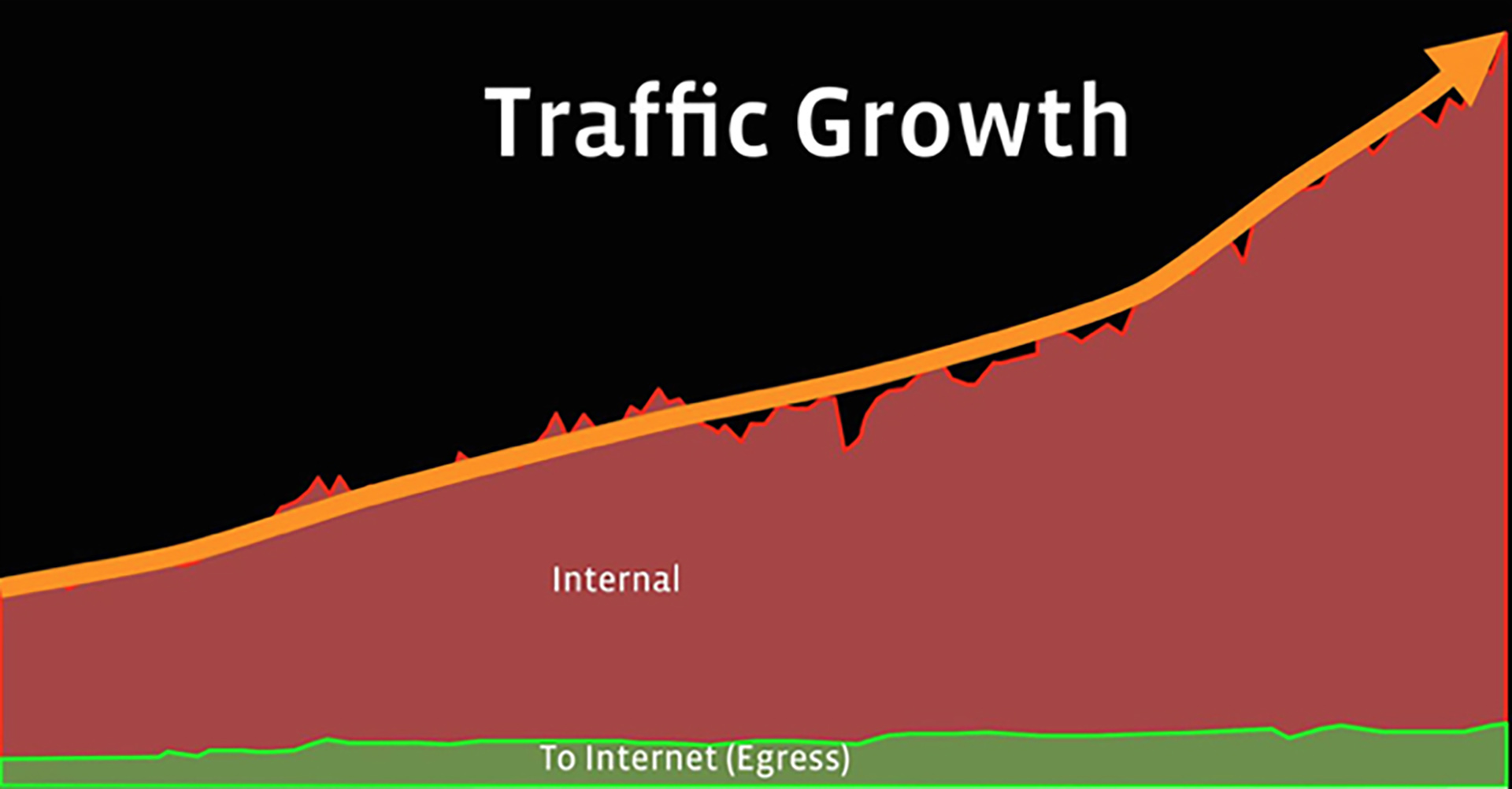
Our production backbone network connects our data centers and delivers content to our users. The network supports a vast number of different services, distributed across a multitude of data centers. Traffic patterns shift over time from one data center to another due to the introduction of new services, service architecture changes, changes in user behavior, new data centers, etc. As a result, we’ve seen exponential and highly variable traffic demands for many years.
To meet service bandwidth expectations we need an accurate long-term demand forecast. However, because of the nature of our services, the fluidity of the workloads, and the difficulty in predicting future service behavior, it is difficult to predict future traffic between each data center pair (i.e., the traffic matrix). To account for this traffic uncertainty, we’ve made design methodology changes that will eliminate our dependence on predicting the future traffic matrix. We achieve this by planning the production network for an aggregate traffic originating from or terminating toward a data center, referred to as network hose. By planning for network hose, we reduce the forecast complexity by an order of magnitude.
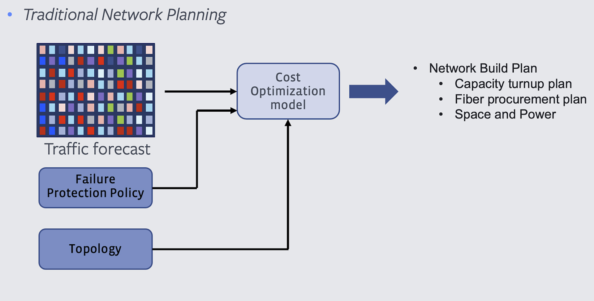
The traditional approach to network planning
The traditional approach to network planning is to size the topology to accommodate a given traffic matrix under a set of potential failures that we define using a failure protection policy. In this approach:
- Traffic matrix is the volume of the traffic we forecast between any two data centers (pairwise demands).
- Failure protection policy is a set of failures that are commonly observed in any large network, such as singular fiber cuts or dual submarine link failures, or a set of failures that have been encountered multiple times in the past (e.g., dual aerial fiber failure outside a data center).
- We use a cost optimization model to calculate the network capacity plan. Essentially, the well-known integer linear programming formulation ensures availability of capacity to service the traffic matrix under all failures that are defined in our policy.
What is the problem?
The following reasons made us rethink the classical approach:
- Lack of long-term fidelity: Backbone network capacity turnup requires longer lead times, typically in the order of months or even years, in the case of procuring or building a terrestrial fiber route or building a submarine cable across the Atlantic Ocean. Given our services’ past growth and dynamic nature, it’s challenging to forecast service behavior for a time frame over six months. Our original approach was to handle traffic uncertainties by dimensioning the network for worst-case assumptions and sizing for a higher percentile, say P95.
- Asking every service owner to provide a traffic estimate per data center pair is hardly manageable. With the traditional approach, a service owner needs to give an explicit demand spec. That is daunting because not only do we see changes in current service behavior, but we also don’t know what new services will be introduced and will consume our network in a one-year or above time frame. The problem of forecasting exact traffic is even more difficult in the long term because the upcoming data centers are not even in production when the forecast is requested.
- Abstracting network as a consumable resource: A service typically requires compute, storage, and network resources to operate from a data center. Each data center has a known compute and storage resource that can be distributed to different services. A service owner can reason the short-term and long-term requirements for these resources and can consider them as a consumable entity per data center. However, this is not true for the network because the network is a shared resource. It is desirable to create a planning method that can abstract the network’s complexity and present it to services like any other consumable entity per data center.
- Operational churn: Tracking every service’s traffic surge, identifying its root cause, and estimating its potential impact is becoming increasingly difficult. Most of these surges are harmless because not all services surge simultaneously. Nonetheless, this still creates operational overhead for tracking many false alarms.
Network-hose planning model:
Instead of forecasting traffic for each (source, destination) pair, we perform a traffic forecast for total egress and total ingress traffic per data center, i.e., network hose. Instead of asking how much traffic a service would generate from X to Y, we ask how much ingress and egress traffic a service is expected to generate from X. Thus, we replace the O(N^2) data points per service with O(N). When planning for aggregated traffic, we naturally bake in statistical multiplexing in the forecast.
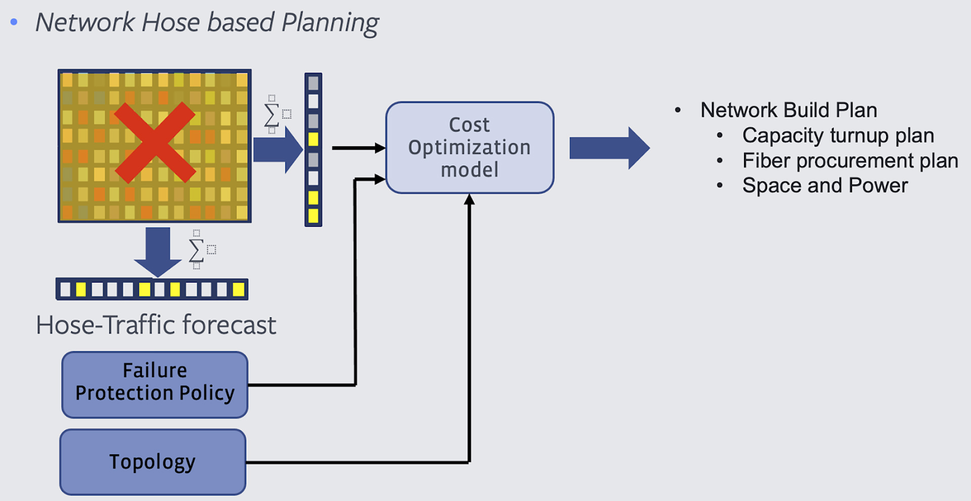
The figure above reflects the change in input for the planning problem. Instead of a classical traffic matrix, we now only have traffic hose forecast and generate a network plan that supports it under all failures defined by the failure policy.
Solving the planning challenge
While the network hose model captures the end-to-end demand uncertainty concisely, it creates a different challenge: Dealing with the many demand sets realizing the hose constraints. In other words, if we take the convex polytope of all the demand sets that satisfy the hose constraint, it has a continuous space inside the polytope to deal with. Typically, this would be useful for an optimization problem as we can leverage linear programming techniques to solve this effectively. However, this model’s key difference is that each point inside the convex polytope is a single traffic matrix. The long-term network build plan has to satisfy all such demand sets if we fulfill the hose constraint. That creates an enormous computational challenge as designing a cross-layer global production network is already an intensive optimization problem for a single demand set.
The above reasons drive the need to intelligently identify a few demand sets from this convex polytope that can serve as reference demand sets for the network design problem. In finding these reference demand sets, we are interested in a few fundamental properties that they should satisfy:
- These are the demand sets that are likely to drive the need for additional resources on the production network (fiber and equipment).
- If we design the network explicitly for this subset, then we would like to guarantee with high probability that we cover the remaining demand sets.
- The number of reference demand sets should be as small as possible to reduce the cross-layer network design problem’s state space.
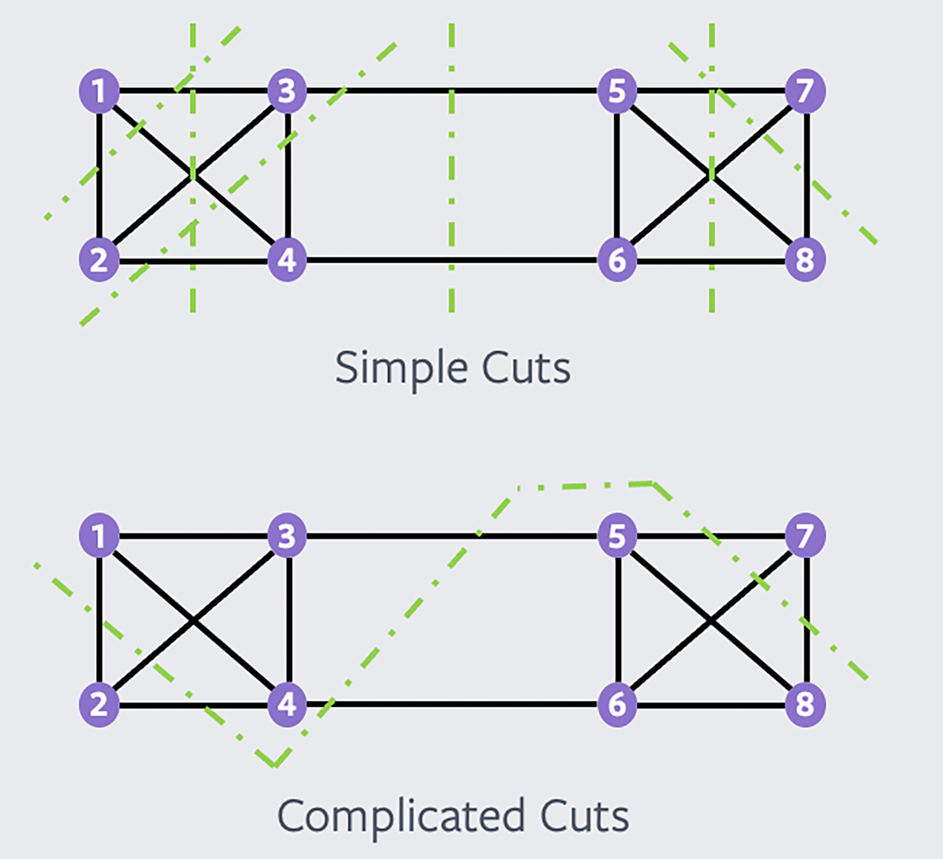
To identify these reference demand sets, we exploit the cuts in the topology and location (latitude, longitude) of the data centers to gain insights into the maximum flow that can cross a network cut. See the example below for a network cut in an example topology. This network cut partitions the topology into two sets of nodes, (1,2,3,4) and (5,6,7,8). To size the link on this network cut, we need only one traffic matrix that generates maximum traffic over the graph cut. All other traffic matrices with lower or equal traffic over this cut get admitted on this with no additional bandwidth requirement over the graph cut.
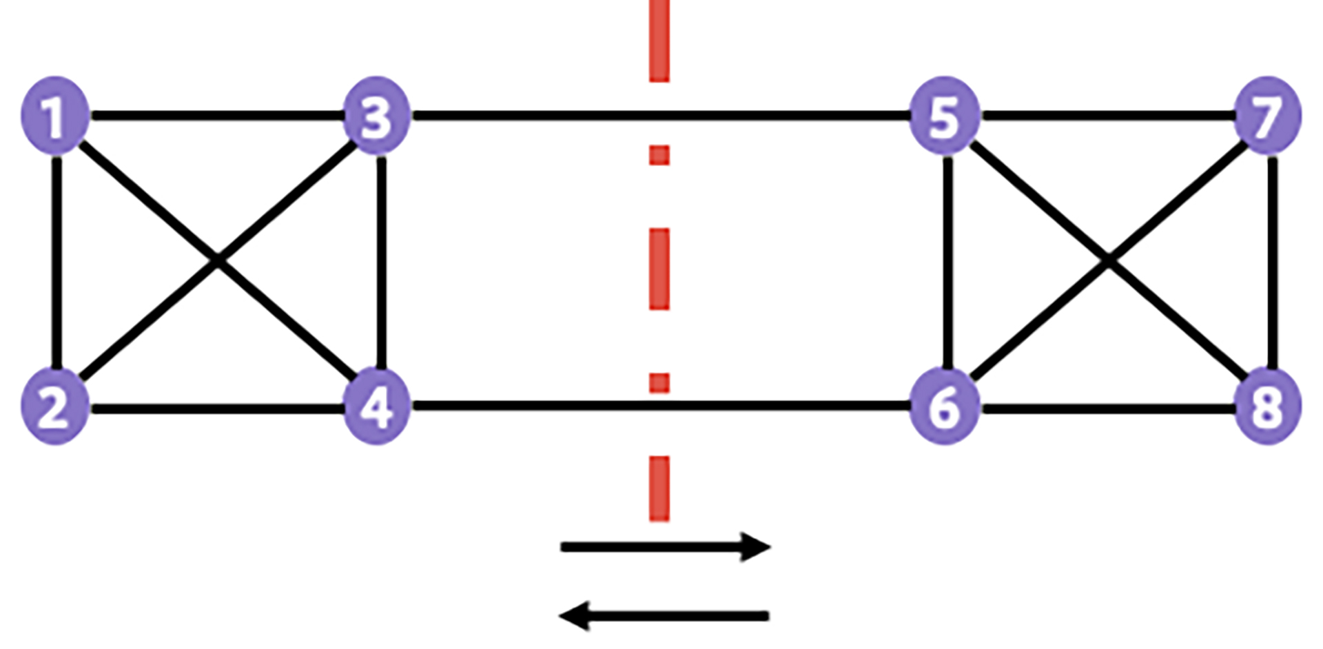
Note that, in a topology with N nodes, we can create 2^N network cuts and have one traffic matrix per cut. However, the geographical nature of these cuts is essential, given the planer nature of our topology. It turns out that simple cuts (typically a straight line cut) are more critical to dimension the topology than more complicated cuts. As shown in the figure below, a traffic matrix for each of the simple cuts is more meaningful than a traffic matrix for the “complicated” cuts: A complicated cut is already taken into account by a set of simple cuts.
By focusing on the simple cuts, we reduce the number of reference demand sets to the smallest traffic matrix set. We solve these traffic matrices using a cost optimization model and produce a network plan supporting all possible traffic matrices. Based on simulations, we observe that given the nature of our topology, additional capacity required to keep the hose-based traffic matrix is not significant but provides powerful simplicity in our planning and operational workflows.
By adopting a hose-based network capacity planning method, we have reduced the forecast complexity by an order of magnitude, enabled services to reason network like any other consumable entity, and simplified operations by eliminating a significant number of traffic surge–related alarms because we now track traffic surge in aggregate from a data center and not surge between every two data centers.
Many people contributed to this project, but we’d particularly like to thank Tyler Price, Alexander Gilgur, Hao Zhong, Ying Zhang, Alexander Nikolaidis, Gaya Nagarajan, Steve Politis, Biao Lu, Ying Zhang, and Abhinav Triguna for being instrumental in making this project happen.


