
Implementing Precision Time Protocol (PTP) at Meta allows us to synchronize the systems that drive our products and services down to nanosecond precision. PTP’s predecessor, Network Time Protocol (NTP), provided us with millisecond precision, but as we scale to more advanced systems on our way to building the next computing platform, the metaverse and AI, we need to ensure that our servers are keeping time as accurately and precisely as possible. With PTP in place, we’ll be able to enhance Meta’s technologies and programs — from communications and productivity to entertainment, privacy, and security — for everyone, across time zones and around the world.
The journey to PTP has been years long, as we’ve had to rethink how both the timekeeping hardware and software operate within our servers and data centers.
We are sharing a deep technical dive into our PTP migration and our innovations that have made it possible
Table of contents |
The case for PTP
Before we dive into the PTP architecture, let’s explore a simple use case for extremely accurate timing, for the sake of illustration.
Imagine a situation in which a client writes data and immediately tries to read it. In large distributed systems, chances are high that the write and the read will land on different back-end nodes.
If the read is hitting a remote replica that doesn’t yet have the latest update, there is a chance the user will not see their own write:
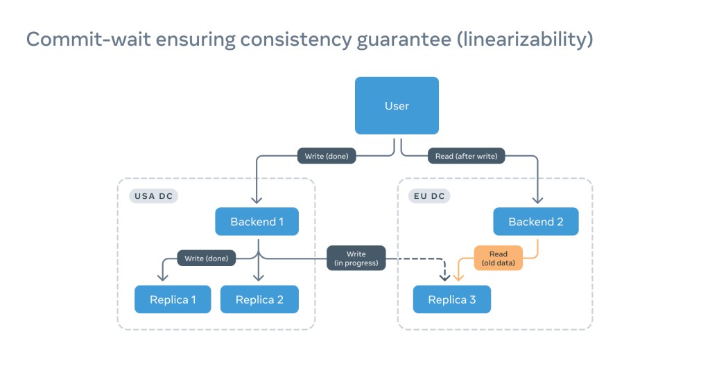
This is annoying at the very least, but more important is that this is violating a linearizability guarantee that allows for interaction with a distributed system in the same way as with a single server.
The typical way to solve this is to issue multiple reads to different replicas and wait for a quorum decision. This not only consumes extra resources but also significantly delays the read because of the long network round-trip delay.
Adding precise and reliable timestamps on a back end and replicas allows us to simply wait until the replica catches up with the read timestamp:
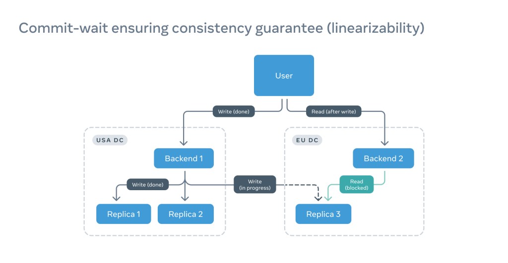
This not only speeds up the read but also saves tons of compute power.
A very important condition for this design to work is that all clocks be in sync or that the offset between a clock and the source of time be known. The offset, however, changes because of constant correction, drifting, or simple temperature variations. For that purpose, we use the notion of a Window of Uncertainty (WOU), where we can say with a high probability where the offset is. In this particular example, the read should be blocked until the read timestamp plus WOU.
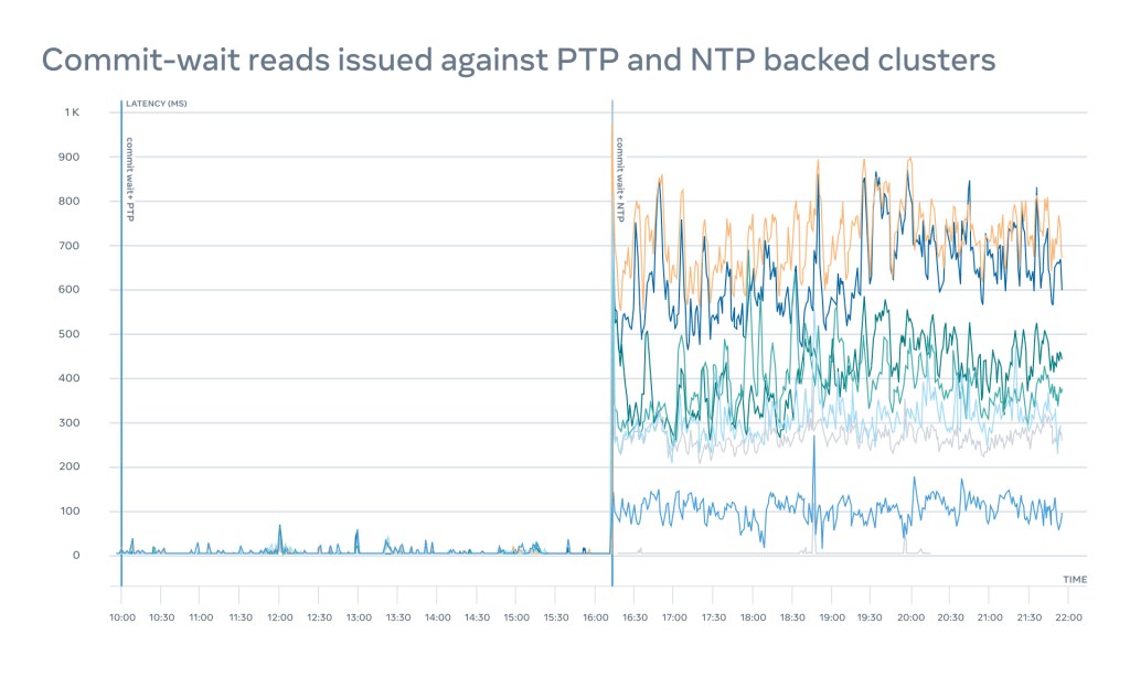
One could argue that we don’t really need PTP for that. NTP will do just fine. Well, we thought that too. But experiments we ran comparing our state-of-the-art NTP implementation and an early version of PTP showed a roughly 100x performance difference:
There are several additional use cases, including event tracing, cache invalidation, privacy violation detection improvements, latency compensation in the metaverse, and simultaneous execution in AI, many of which will greatly reduce hardware capacity requirements. This will keep us busy for years ahead.
Now that we are on the same page, let’s see how we deployed PTP at Meta scale.
The PTP architecture
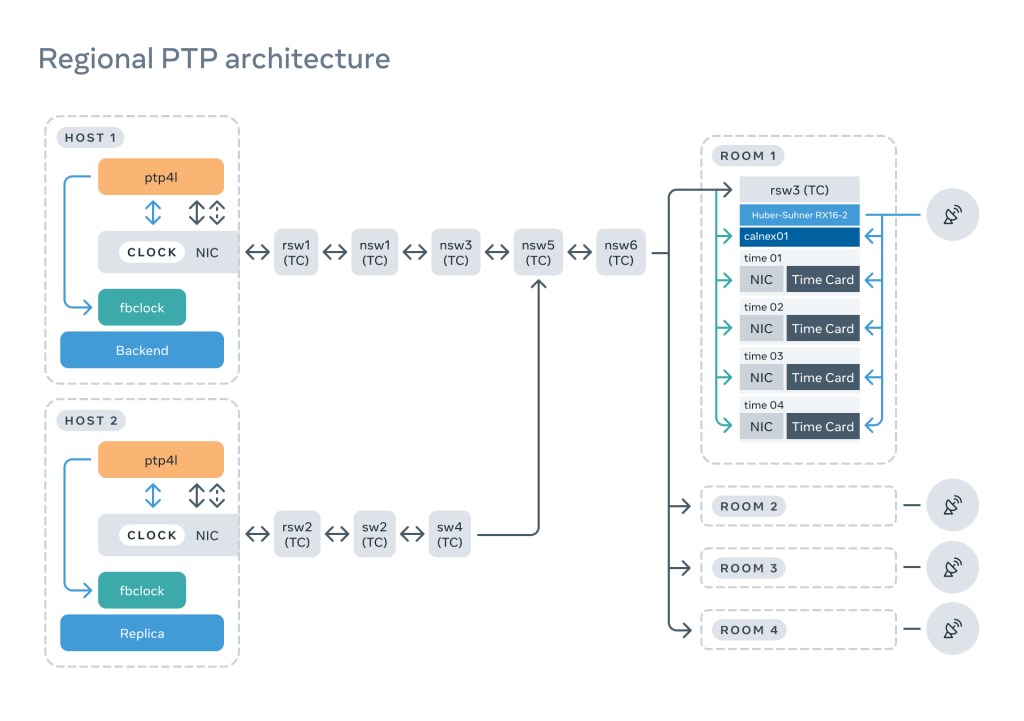
After several reliability and operational reviews, we landed on a design that can be split into three main components: the PTP rack, the network, and the client.
Buckle up — we are going for a deep dive.
The PTP rack
This houses the hardware and software that serves time to clients; the rack consists of multiple critical components, each of which has been carefully selected and tested.
The antenna
The GNSS antenna is easily one of the least appreciated components. But this is the place where time originates, at least on Earth.
We’re striving for nanosecond accuracy. And if the GNSS receiver can’t accurately determine the position, it will not be able to calculate time. We have to strongly consider the signal-to-noise ratio (SNR). A low-quality antenna or obstruction to the open sky can result in a high 3D location standard deviation error. For time to be determined extremely accurately, GNSS receivers should enter a so-called time mode, which typically requires a <10m 3D error.
It’s absolutely essential to ensure an open sky and install a solid stationary antenna. We also get to enjoy some beautiful views:
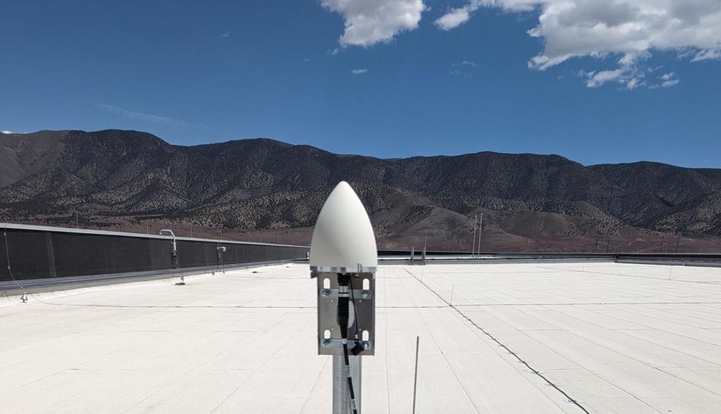
While we were testing different antenna solutions, a relatively new GNSS-over-fiber technology got our attention. It’s free from almost all disadvantages — it doesn’t conduct electricity because it’s powered by a laser via optical fiber, and the signal can travel several kilometers without amplifiers.
Inside the building, it can use pre-existing structured fiber and LC patch panels, which significantly simplifies the distribution of the signal. In addition, the signal delays for optical fiber are well defined at approximately 4.9ns per meter. The only thing left is the delay introduced by the direct RF to laser modulation and the optical splitters, which are around 45ns per box.
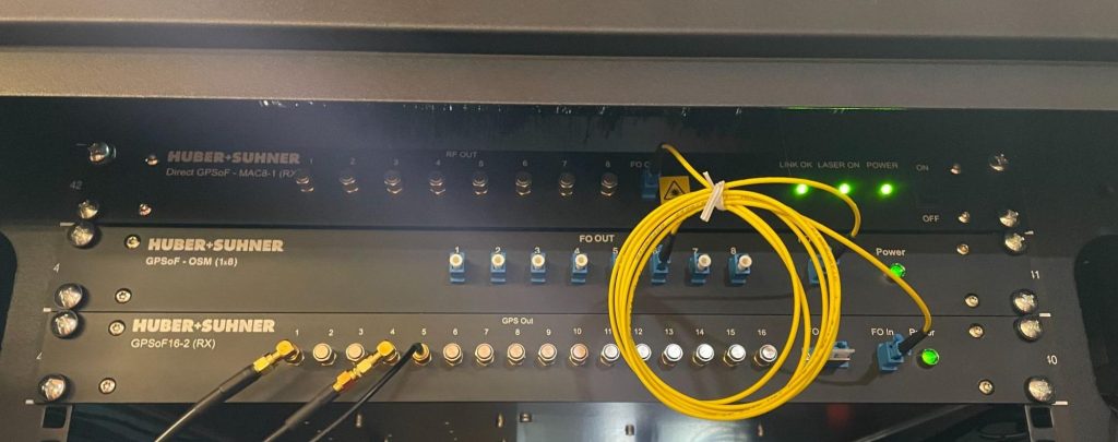
By conducting tests, we confirmed that the end-to-end antenna delay is deterministic (typically about a few hundred nanoseconds) and can easily be compensated on the Time Appliance side.
Time Appliance
The Time Appliance is the heart of the timing infrastructure. This is where time originates from the data center infrastructure point of view. In 2021, we published an article explaining why we developed a new Time Appliance and why existing solutions wouldn’t cut it.
But this was mostly in the context of NTP. PTP, on the other hand, brings even higher requirements and tighter constraints. Most importantly, we made a commitment to reliably support up to 1 million clients per appliance without hurting accuracy and precision. To achieve this, we took a critical look at many of the traditional components of the Time Appliance and thought really hard about their reliability and diversity.
The Time Card
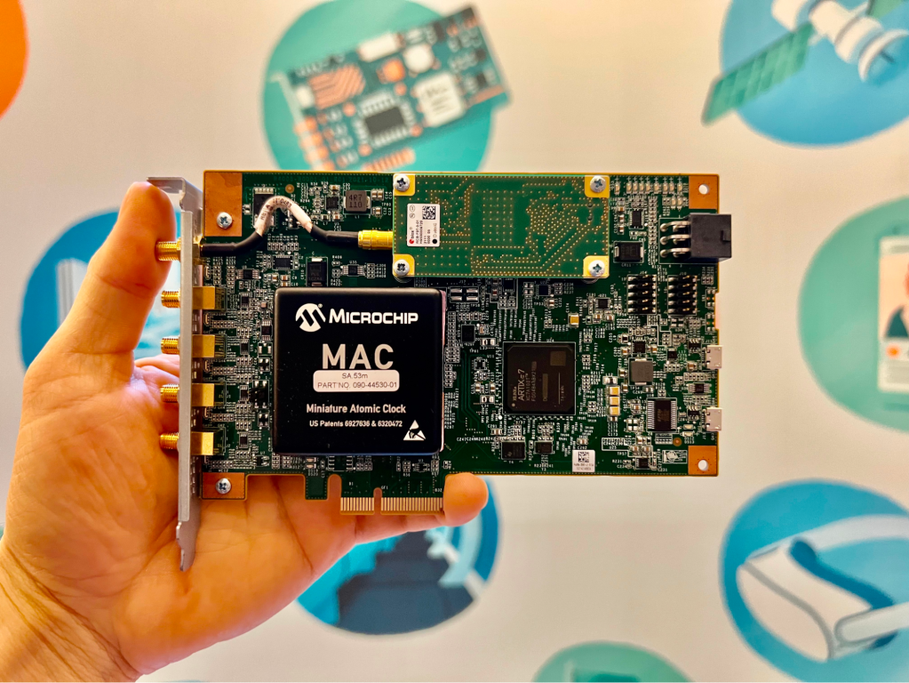
To protect our infrastructure from a critical bug or a malicious attack,we decided to start diversification from the source of time — the Time Card. Last time, we spoke a lot about the Time Card design and the advantages of an FPGA-based solution. Under the Open Compute Project (OCP), we are collaborating with vendors such as Orolia, Meinberg, Nvidia, Intel, Broadcom, and ADVA, which are all implementing their own time cards, matching the OCP specification.
Oscillatord
The Time Card is a critical component that requires special configuration and monitoring. For this purpose, we worked with Orolia to develop a disciplining software, called oscillatord, for different flavors of the Time Cards. This has become the default tool for:
- GNSS receiver configuration: setting the default config, and adjusting special parameters like antenna delay compensation. It also allows the disabling of any number of GNSS constellations to simulate a holdover scenario.
- GNSS receiver monitoring: reporting number of satellites, GNSS quality, availability of different constellations, antenna status, leap second, etc.
- Atomic clock configuration: Different atomic clocks require different configuration and sequence of events. For example, it supports SA53 TAU configuration for fast disciplining, and with mRO-50, it supports a temperature-to-frequency relation table.
- Atomic clock monitoring: Parameters such as a laser temperature and lock have to be monitored thoroughly, and fast decisions must be made when the values are outside of operational range.
Effectively, the data exported from oscillatord allows us to decide whether the Time Appliance should take traffic or should be drained.
Network card
Our ultimate goal is to make protocols such as PTP propagate over the packet network. And if the Time Card is the beating heart of the Time Appliance, the network card is the face. Every time-sensitive PTP packet gets hardware timestamped by the NIC. This means the PTP Hardware Clock (PHC) of the NIC must be accurately disciplined.
If we simply copy the clock values from Time Card to the NIC, using the phc2sys or a similar tool, the accuracy will not be nearly enough. In fact, our experiments show that we would easily lose ~1–2 microseconds while going through PCIe, CPU, NUMA, etc. The performance of synchronization over PCIe bus will dramatically improve with the emerging Precision Time Measurement (PTM) technology, as the development and support for various peripherals with this capability is in progress.
For our application, since we use NICs with PPS-in capabilities, we employed ts2phc, which copies clock values at first and then aligns the clock edges based on a pulse per second (PPS) signal. This requires an additional cable between the PPS output of the Time Card and the PPS input of the NIC, as shown in the picture below.
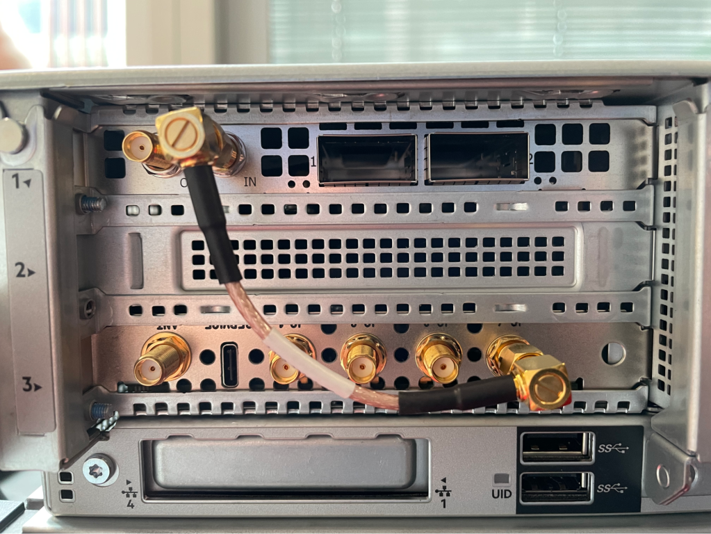
We constantly monitor offset and make sure it never goes out of a ±50ns window between the Time Card and the NIC:
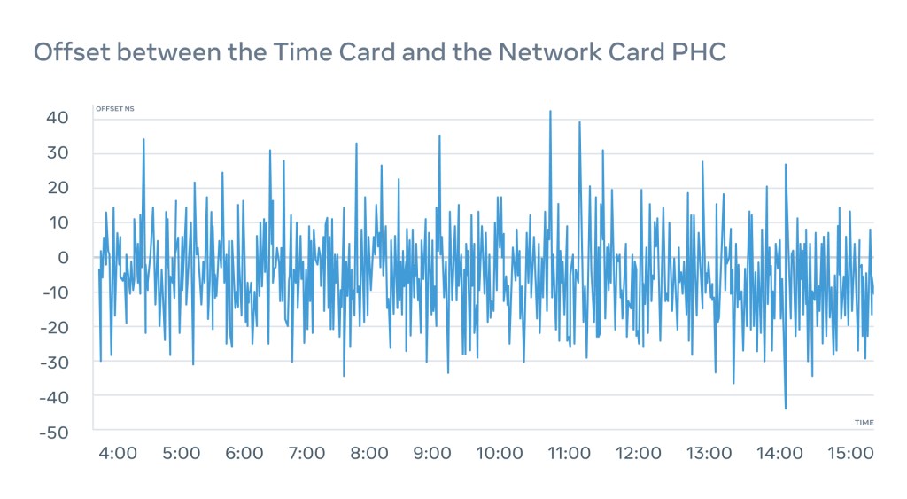
We also monitor the PPS-out interface of the NIC to act as a fail-safe and ensure that we actually know what’s going on with the PHC on the NIC.
ptp4u
While evaluating different preexisting PTP server implementations, we experienced scalability issues with both open source and closed proprietary solutions, including the FPGA-accelerated PTP servers we evaluated. At best, we could get around 50K clients per server. At our scale, this means we would have to deploy many racks full of these devices.
Since PTP’s secret sauce is the use of hardware timestamps, the server implementation doesn’t have to be a highly optimized C program or even an FPGA-accelerated appliance.
We implemented a scalable PTPv2 unicast PTP server in Go, which we named ptp4u, and open-sourced it on GitHub. With some minor optimizations, we were able to support over 1 million concurrent clients per device, which was independently verified by an IEEE 1588v2 certified device.
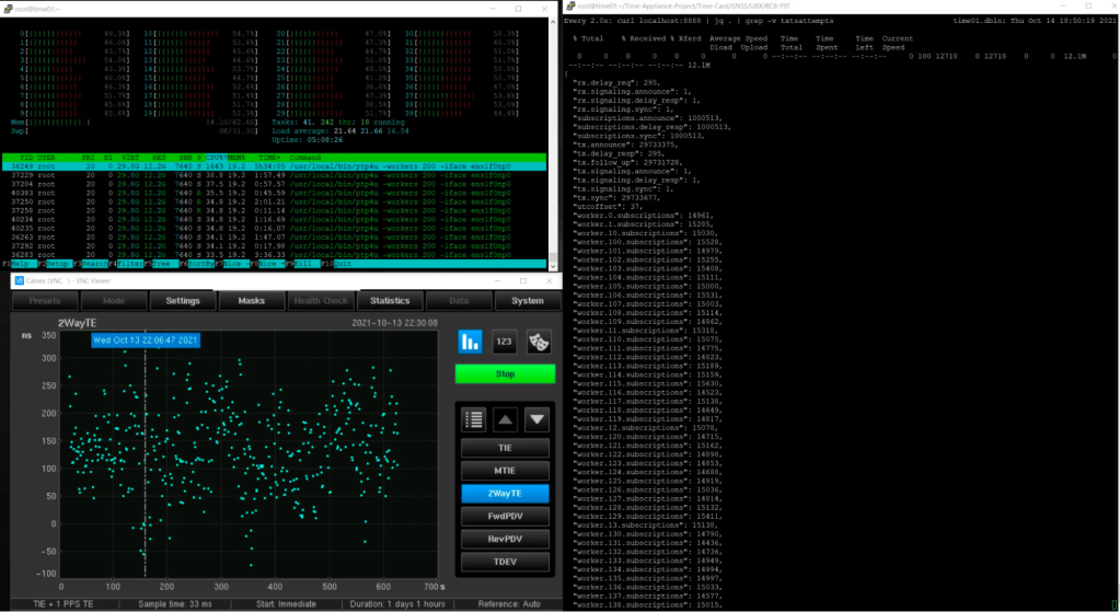
This was possible through the simple but elegant use of channels in Go that allowed us to pass subscriptions around between multiple powerful workers.
Because ptp4u runs as a process on a Linux machine, we automatically get all the benefits, like IPv6 support, firewall, etc., for free.
c4u
The ptp4u server has many configuration options, allowing it to pass dynamically changing parameters such as PTP Clock Accuracy, PTP Clock Class, and a UTC offset — that is currently set to 37 seconds (we’re looking forward this becoming a constant) — down to clients.
In order to frequently generate these parameters, we implemented a separate service called c4u, which constantly monitors several sources of information and compiles the active config for ptp4u:
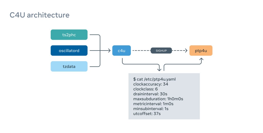
This gives us flexibility and reactivity if the environment changes. For example, if we lose the GNSS signal on one of the Time Appliances, we will switch the ClockClass to HOLDOVER and clients will immediately migrate away from it. It is also calculating ClockAccuracy from many different sources, such as ts2phc synchronization quality, atomic clock status, and so on.
We calculate the UTC offset value based on the content of the tzdata package because we pass International Atomic Time (TAI) down to the clients.
Calnex Sentinel
We wanted to make sure our Time Appliances are constantly and independently assessed by a well-established certified monitoring device. Luckily, we’ve already made a lot of progress in the NTP space with Calnex, and we were in a position to apply a similar approach to PTP.
We collaborated with Calnex to take their field device and repurpose it for data center use, which involved changing the physical form factor and adding support for features such as IPv6.
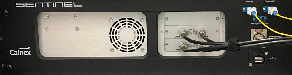
We connect the Time Appliance NIC PPS-out to the Calnex Sentinel, which allows us to monitor the PHC of the NIC with nanosecond accuracy.
We will explore monitoring in great detail in “How we monitor the PTP architecture,” below.
The PTP network
PTP protocol
The PTP protocol supports the use of both unicast and multicast modes for the transmission of PTP messages. For large data center deployments, unicast is preferred over multicast because it significantly simplifies network design and software requirements.
Let’s take a look at a typical PTP unicast flow:
A client starts the negotiation (requesting unicast transmission). Therefore, it must send:
- A Sync Grant Request (“Hey server, please send me N Sync and Follow-Up messages per second with the current time for the next M minutes”)
- An Announce Grant Request (“Hey server, please send me X Announce messages per second with your status for the next Y minutes”)
- A Delay Response Grant Request (“Hey server, I am going to send you Delay Requests — please respond with Delay Response packets for the next Z minutes”)
- The server needs to grant these requests and send grant responses.
- Then the server needs to start executing subscriptions and sending PTP messages.
- All subscriptions are independent of one another.
- It’s on the server to obey the send interval and terminate the subscription when it expires. (PTP was originally multicast only, and one can clearly see the multicast origin in this design).
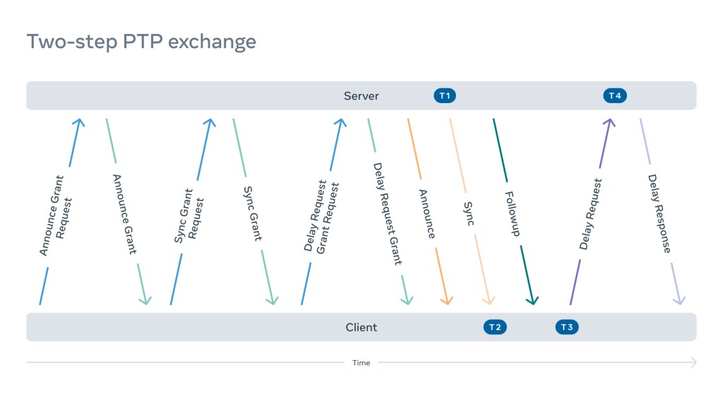
- In two-step configuration, when the server sends Sync messages, it has to read the TX hardware timestamp and send a Follow-Up message containing that timestamp.
- The client will send Delay Requests within the agreed-upon interval to determine the path delay. The server needs to read the RX hardware timestamp and return it to the client.
- The client needs to periodically refresh the grant, and the process repeats.
Schematically (just for the illustration), it will look like this:
Transparent clocks
We initially considered leveraging boundary clocks in our design. However, boundary clocks come with several disadvantages and complications:
- You need network equipment or some special servers to act as a boundary clock.
- A boundary clock acts as a time server, creating greater demand for short-term stability and holdover performance.
- Since the information has to pass through the boundary clocks from the time servers down to the clients, we would have to implement special support for this.
To avoid this additional complexity, we decided to rely solely on PTP transparent clocks.
Transparent clocks (TCs) enable clients to account for variations in network latency, ensuring a much more precise estimation of clock offset. Each data center switch in the path between client and time server reports the time each PTP packet spends transiting the switch by updating a field in the packet payload, the aptly named Correction Field (CF).
PTP clients (also referred to as ordinary clocks, or OCs) calculate network mean path delay and clock offsets to the time servers (grandmaster clocks, or GMs) using four timestamps (T1, T2, T3, and T4) and two correction field values (CFa and CFb), as shown in the diagram below:
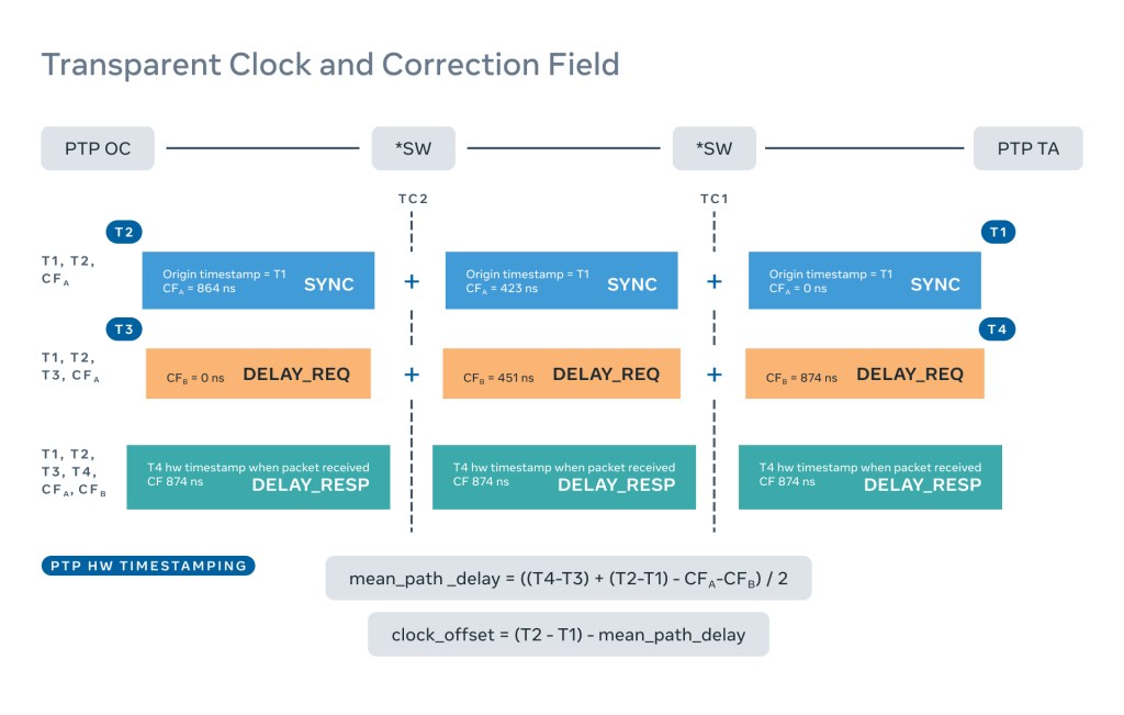
- T1 is the hardware timestamp when the SYNC packet is sent by the Time Server.
- T2 is the hardware timestamp when the OC receives the SYNC packet.
- CFa is the sum of the switch delays recorded by each switch (TC) in the path from time server to the client (for SYNC packet).
- T3 is the hardware timestamp the delay request is sent by the Client.
- T4 is the hardware timestamp when the time server receives the delay request.
- CFb is the sum of the switch delays recorded by each switch in the path from the Client to the time server (for Delay Request packet).
To understand the impact of just one disabled transparent clock on the way between client and a server, we can examine the logs:
We can see the path delay explodes, sometimes even becoming negative which shouldn’t happen during normal operations. This has a dramatic impact on the offset, moving it from ±100 nanoseconds to -400 microseconds (over 4000 times difference). And the worst thing of all, this offset will not even be accurate, because the mean path delay calculations are incorrect.
According to our experiments, modern switches with large buffers can delay packets for up to a couple of milliseconds which will result in hundreds of microseconds of a path delay calculation error. This will drive the offset spikes and will be clearly visible on the graphs:
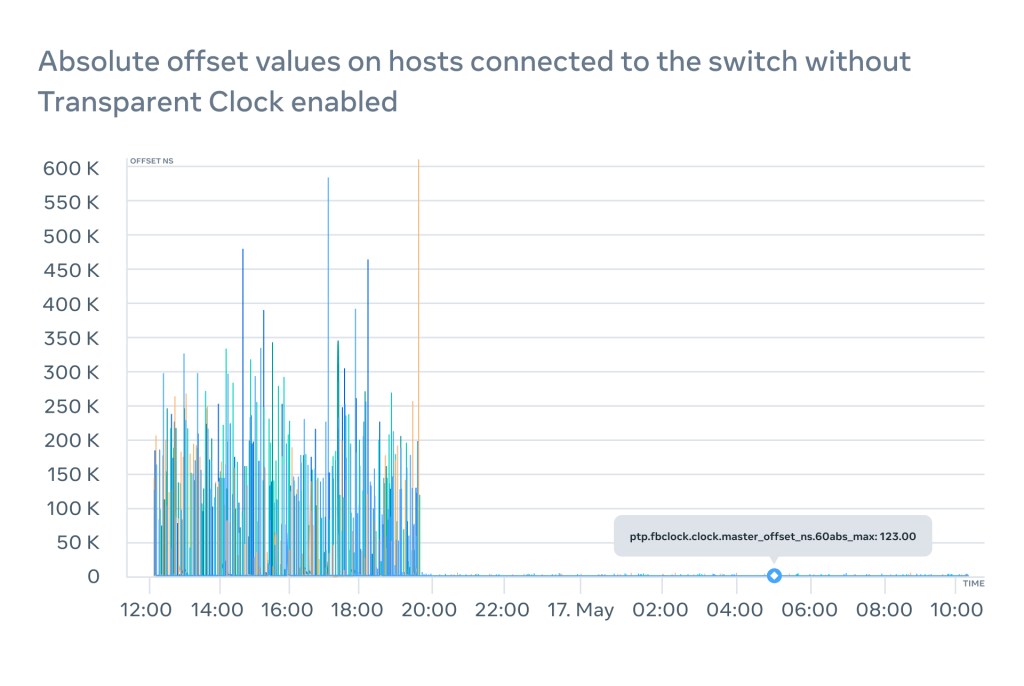
The bottom line is that running PTP in datacenters in the absence of TCs leads to unpredictable and unaccountable asymmetry in the roundtrip time. And the worst of all – there will be no simple way to detect this. 500 microseconds may not sound like a lot, but when customers expect a WOU to be several microseconds, this may lead to an SLA violation.
The PTP Client
Timestamps
Timestamping the incoming packet is a relatively old feature supported by the Linux kernel for decades. For example software (kernel) timestamps have been used by NTP daemons for years. It’s important to understand that timestamps are not included into the packet payload by default and if required, must be placed there by the user application.
Reading RX timestamp from the user space is a relatively simple operation. When packet arrives, the network card (or a kernel) will timestamp this event and include the timestamp into the socket control message, which is easy to get along with the packet itself by calling a recvmsg syscall with MSG_ERRQUEUE flag set.
| 128 bits | 64 bits | 64 bits | 64 bits |
| Socket control message header | Software Timestamp | Legacy Timestamp | Hardware Timestamp |
For the TX Hardware timestamp it’s a little more complicated. When sendto syscall is executed it doesn’t lead to an immediate packet departure and neither to a TX timestamp generation. In this case the user has to poll the socket until the timestamp is accurately placed by the kernel. Often we have to wait for several milliseconds which naturally limits the send rate.
Hardware timestamps are the secret sauce that makes PTP so precise. Most of the modern NICs already have hardware timestamps support where the network card driver populates the corresponding section.
It’s very easy to verify the support by running the ethtool command:
$ ethtool -T eth0
Time stamping parameters for eth0:
Capabilities:
	hardware-transmit
	hardware-receive
	hardware-raw-clock
PTP Hardware Clock: 0
Hardware Transmit Timestamp Modes:
	off
	on
Hardware Receive Filter Modes:
	none
	All
It’s still possible to use PTP with software (kernel) timestamps, but there won’t be any strong guarantees on their quality, precision, and accuracy.
We evaluated this possibility as well and even considered implementing a change in the kernel for “faking” the hardware timestamps with software where hardware timestamps are unavailable. However, on a very busy host we observed the precision of software timestamps jumped to hundreds of microseconds and we had to abandon this idea.
ptp4l
ptp4l is an open source software capable of acting as both a PTP client and a PTP server. While we had to implement our own PTP server solution for performance reasons, we decided to stick with ptp4l for the client use case.
Initial tests in the lab revealed that ptp4l can provide excellent synchronization quality out of the box and align time on the PHCs in the local network down to tens of nanoseconds.
However, as we started to scale up our setup some issues started to arise.
Edge cases
In one particular example we started to notice occasional “spikes” in the offset. After a deep dive we identified fundamental hardware limitations of one of the most popular NICs on the market:
- The NIC has only a timestamp buffer for 128 packets.
- The NIC is unable to distinguish between PTP packets (which need a hardware timestamp) and other packets which don’t.
This ultimately led to the legitimate timestamps being displaced by timestamps coming from other packets. But what made things a lot worse – the NIC driver tried to be overly clever and placed the software timestamps in the hardware timestamp section of the socket control message without telling anyone.
It’s a fundamental hardware limitation affecting a large portion of the fleet which is impossible to fix.
We had to implement an offset outliers filter, which changed the behavior of PI servo and made it stateful. It resulted in occasional outliers being discarded and the mean frequency set during the micro-holdover:
If not for this filter, ptp4l would have steered PHC frequency really high, which would result in several seconds of oscillation and bad quality in the Window of Uncertainty we generate from it.
Another issue arose from the design of BMCA. The purpose of this algorithm is to select the best Time Appliance when there are several to choose from in the ptp4l.conf. It does by comparing several attributes supplied by Time Servers in Announce messages:
- Priority 1
- Clock Class
- Clock Accuracy
- Clock Variance
- Priority 2
- MAC Address
The problem manifests itself when all aforementioned attributes are the same. BMCA uses Time ApplianceMAC address as the tiebreaker which means under normal operating conditions one Time Server will attract all client traffic.
To combat this, we introduced a so-called “sharding” with different PTP clients being allocated to different sub-groups of Time Appliances from the entire pool.
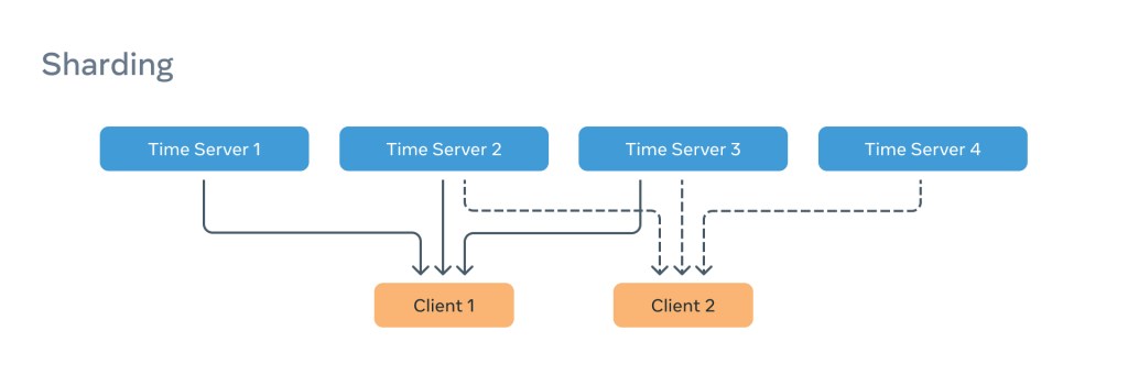
This only partially addressed the issue with one server in each subgroup taking the entire load for that grouping. The solution was to enable clients to express a preference, and so we introduced Priority3 into the selection criteria just above the MAC address tiebreaker. This means that clients configured to use the same Time Appliances can prefer different servers.
Client 1:
[unicast_master_table]
UDPv6 time_server1 1
UDPv6 time_server2 2
UDPv6 time_server3 3
Client 2:
[unicast_master_table]
UDPv6 time_server2 1
UDPv6 time_server3 2
UDPv6 time_server1 3
This ensures we can distribute load evenly across all Time Appliances under normal operating conditions.
Another major challenge we faced was ensuring PTP worked with multi-host NICs – multiple hosts sharing the same physical network interface and therefore a single PHC. However, ptp4l has no knowledge of this and tries to discipline the PHC like there are no other neighbors.
Some NIC manufacturers developed a so-called “free running” mode where ptp4l is just disciplining the formula inside the kernel driver. The actual PHC is not affected and keeps running free. This mode results in a slightly worse precision, but it’s completely transparent to ptp4l.
Other NIC manufacturers only support a “real time clock” mode, when the first host to grab the lock actually disciplines the PHC. The advantage here is a more precise calibration and higher quality holdover, but it leads to a separate issue with ptp4l running on the other hosts using the same NIC as attempts to tune PHC frequency have no impact, leading to inaccurate clock offset and frequency calculations.
PTP profile
To describe the datacenter configuration, we’ve developed and published a PTP profile, which reflects the aforementioned edge cases and many more.
Alternative PTP clients (updated: 2/2024)
We are evaluating the possibility of using an alternative PTP client. Our main criteria are:
- Support our PTP profile
- Meets our synchronization quality requirements
- Open source
After much consideration and evaluation of several alternative PTP clients we’ve decided to develop and open source a high-performance Simple PTP (SPTP) client. Our own tests with SPTP have show comparable performance to PTP, but with significant improvements in CPU, memory, and network utilization.
Continuously incrementing counter
In the PTP protocol, it doesn’t really matter what time we propagate as long as we pass a UTC offset down to the clients. In our case, it’s International Atomic Time (TAI), but some people may choose UTC. We like to think about the time we provide as a continuously incrementing counter.
At this point we are not disciplining the system clock and ptp4l is solely used to discipline the NIC’s PHC.
fbclock
Synchronizing PHCs across the fleet of servers is good, but it’s of no benefit unless there is a way to read and manipulate these numbers on the client.
For this purpose, we developed a simple and lightweight API called fbclock that gathers information from PHC and ptp4l and exposes easy digestible Window Of Uncertainty information:
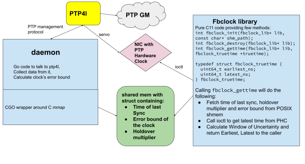
Through a very efficient ioctl PTP_SYS_OFFSET_EXTENDED, fbclock gets a current timestamps from the PHC, latest data from ptp4l and then applies math formula to calculate the Window Of Uncertainty (WOU):
$ ptpcheck fbclock
{"earliest_ns":1654191885711023134,"latest_ns":1654191885711023828,"wou_ns":694}
As you may see, the API doesn’t return the current time (aka time.Now()). Instead, it returns a window of time which contains the actual time with a very high degree of probability In this particular example, we know our Window Of Uncertainty is 694 nanoseconds and the time is between (TAI) Thursday June 02 2022 17:44:08:711023134 and Thursday June 02 2022 17:44:08:711023828.
This approach allows customers to wait until the interval is passed to ensure exact transaction ordering.
Error bound measurement
Measuring the precision of the time or (Window Of Uncertainty) means that alongside the delivered time value, a window (a plus/minus value) is presented that is guaranteed to include the true time to a high level of certainty.
How certain we need to be is determined by how critical it is that the time be correct and this is driven by the specific application.
In our case, this certainty needs to be better than 99.9999% (6-9s). At this level of reliability you can expect less than 1 error in 1,000,000 measurements.
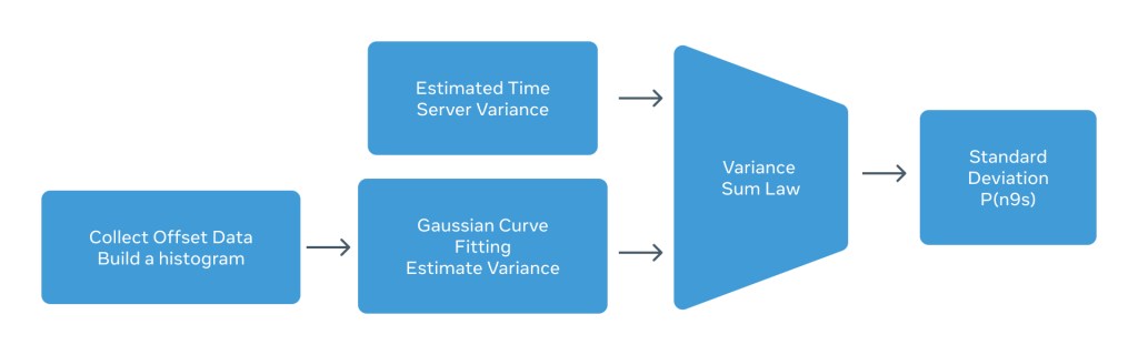
The error rate estimation uses observation of the history of the data (histogram) to fit a probability distribution function (PDF). From the probability distribution function one can calculate the variance (take a root square and get the standard deviation) and from there it will be simple multiplication to get to the estimation of the distribution based on its value.
Below is a histogram taken from the offset measurement from ptp4l running on the ordinary clock.
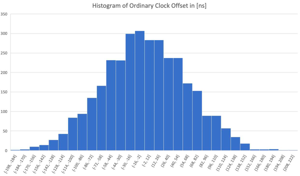
To estimate the total variance (E2E) it is necessary to know the variance of the time error accumulated by the time server all the way to the end node NIC. This includes GNSS, atomic clock, and Time Card PHC to NIC PHC (ts2phc). The manufacturer provides the GNSS error variance. In the case of the UBX-F9T it is about 12 nanoseconds. For the atomic clock the value depends on the disciplining threshold that we’ve set. The tighter the disciplining threshold, the smaller offset variance but lower holdover performance. At the time of running this experiment, the error variance of the atomic clock has been measured to 43ns (standard deviation, std). Finally, the tool ts2phc increases the variance by 30ns (std) resulting in a total variance of 52ns.
The observed results matches the calculated variance obtained by the “Sum of Variance Law.”
According to the sum of variance law, all we need to do is to add all the variance. In our case, we know that the total observer E2E error (measured via the Calnex Sentinel) is about 92ns.
On the other hands for our estimation, we can have the following:
Estimated E2E Variance = [GNSS Variance + MAC Variance + ts2phc Variance] + [PTP4L Offset Variance] = [Time Server Variance] + [Ordinary Clock Variance]
Plugging in the values:
Estimated E2E Variance = (12ns 2) + (43ns2) + (52ns2) + (61ns2) = 8418, which corresponds to 91.7ns
These results show that by propagating the error variance down the clock tree, the E2E error variance can be estimated with a good accuracy. The E2E error variance can be used to calculate the Window Of Uncertainty (WOU) based on the following table.
Simply, by multiplying the estimated E2E error variance in 4.745 we can estimate the Window Of Uncertainty for the probability of 6-9s.
For our given system the probability of 6-9s is about 92ns x 4.745 = 436ns
This means that given a reported time by PTP, considering a window size of 436ns around value guarantees to include the true time by a confidence of over 99.9999%.
Compensation for holdover
While all the above looks logical and great, there is a big assumption there. The assumption is that the connection to the open time server (OTS) is available, and everything is in normal operation mode. A lot of things can go wrong such as the OTS going down, switch going down, Sync messages not behaving as they are supposed to, something in between decides to wake up the on-calls etc. In such a situation the error bound calculation should enter the holdover mode. The same things apply to the OTS when GNSS is down. In such a situation the system will increase the Window Of Uncertainty based on a compound rate. The rate will be estimated based on the stability of the oscillator (scrolling variance) during normal operations. On the OTS the compound rate gets adjusted by the accurate telemetry monitoring of the system (Temperature, Vibration, etc). There is a fair amount of work in terms of calibrating coefficients here and getting to the best outcome and we are still working on those fine tunings.
During the periods of network synchronization availability, the servo is constantly adjusting the frequency of the local clock on the client side (assuming the initial stepping resulted in convergence). A break in the network synchronization (from losing connection to the time server or the time server itself going down) will leave the servo with a last frequency correction value. As a result, such value is not aimed to be an estimation of precision of the local clock but instead a temporary frequency adjustment to reduce the time error (offset) measured between the cline and the time server.
Therefore, it is necessary to first account for synchronization loss periods and use the best estimation of frequency correction (usually, the scrolling average of previous correction values) and second, account for the error bound increase by looking at the last correction value and comparing it with the scrolling average of previous correction values.
How we monitor the PTP architecture
Monitoring is one of the most important parts of the PTP architecture. Due to the nature and impact of the service, we’ve spent quite a bit of time working on the tooling.
Calnex
We worked with the Calnex team to create the Sentinel HTTP API, which allows us to manage, configure, and export data from the device. At Meta, we created and open-sourced an API command line tool allowing human and script friendly interactions.
Using Calnex Sentinel 2.0 we are able to monitor three main metrics per time appliance — NTP, PTP, and PPS.
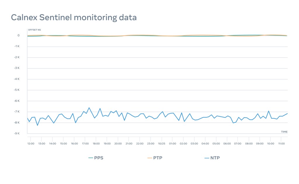
This allows us to notify engineers about any issue with the appliances and precisely detect where the problem is.
For example, in this case both PTP and PPS monitoring resorts in a roughly less than 100 nanosecond variation over 24 hours when NTP stays within 8 microseconds.
ptpcheck
In order to monitor our setup, we implemented and open-sourced a tool called ptpcheck. It has many different subcommands, but the most interesting are the following:
diag
Client subcommand provides an overall status of a ptp client. It reports the time of receipt of last Sync message, clock offset to the selected time server, mean path delay, and other helpful information:
$ ptpcheck diag
[ OK ] GM is present
[ OK ] Period since last ingress is 972.752664ms, we expect it to be within 1s
[ OK ] GM offset is 67ns, we expect it to be within 250µs
[ OK ] GM mean path delay is 3.495µs, we expect it to be within 100ms
[ OK ] Sync timeout count is 1, we expect it to be within 100
[ OK ] Announce timeout count is 0, we expect it to be within 100
[ OK ] Sync mismatch count is 0, we expect it to be within 100
[ OK ] FollowUp mismatch count is 0, we expect it to be within 100
fbclock
Client subcommand that allows querying of an fbclock API and getting a current Window of Uncertainty:
$ ptpcheck fbclock
{"earliest_ns":1654191885711023134,"latest_ns":1654191885711023828,"wou_ns":694}
sources
Chrony-style client monitoring, allows to see all Time Servers configured in the client configuration file, their status, and quality of time.
$ ptpcheck sources
+----------+----------------------+--------------------------+-----------+--------+----------+---------+------------+-----------+--------------+
| SELECTED |       IDENTITY       |         ADDRESS          |   STATE   | CLOCK  | VARIANCE |  P1:P2  | OFFSET(NS) | DELAY(NS) |  LAST SYNC   |
+----------+----------------------+--------------------------+-----------+--------+----------+---------+------------+-----------+--------------+
| true     | abcdef.fffe.111111-1 | time01.example.com.      | HAVE_SYDY | 6:0x22 | 0x59e0   | 128:128 |         27 |      3341 | 868.729197ms |
| false    | abcdef.fffe.222222-1 | time02.example.com.      | HAVE_ANN  | 6:0x22 | 0x59e0   | 128:128 |            |           |              |
| false    | abcdef.fffe.333333-1 | time03.example.com.      | HAVE_ANN  | 6:0x22 | 0x59e0   | 128:128 |            |           |              |
+----------+----------------------+--------------------------+-----------+--------+----------+---------+------------+-----------+--------------+
oscillatord
Server subcommand, allows to read a summary from the Time Card.
$ ptpcheck oscillatord
Oscillator:
	model: sa5x
	fine_ctrl: 328
	coarse_ctrl: 10000
	lock: true
	temperature: 45.33C
GNSS:
	fix: Time (3)
	fixOk: true
	antenna_power: ON (1)
	antenna_status: OK (2)
	leap_second_change: NO WARNING (0)
	leap_seconds: 18
	satellites_count: 28
	survey_in_position_error: 1
Clock:
	class: Lock (6)
	offset: 1
For example, we can see that the last correction on the Time Card was just 1 nanosecond.
phcdiff
This subcommand allows us to get a difference between any two PHCs:
$ ptpcheck phcdiff -a /dev/ptp0 -b /dev/ptp2
PHC offset: -15ns
Delay for PHC1: 358ns
Delay for PHC2: 2.588µs
In this particular case the difference between Time Card and a NIC on a server is -15 nanoseconds.
Client API
It’s good to trigger monitoring periodically or on-demand, but we want to go even further. We want to know what the client is actually experiencing. To this end, we embedded several buckets right inside of the fbclock API based on atomic counters, which increment every time the client makes a call to an API:
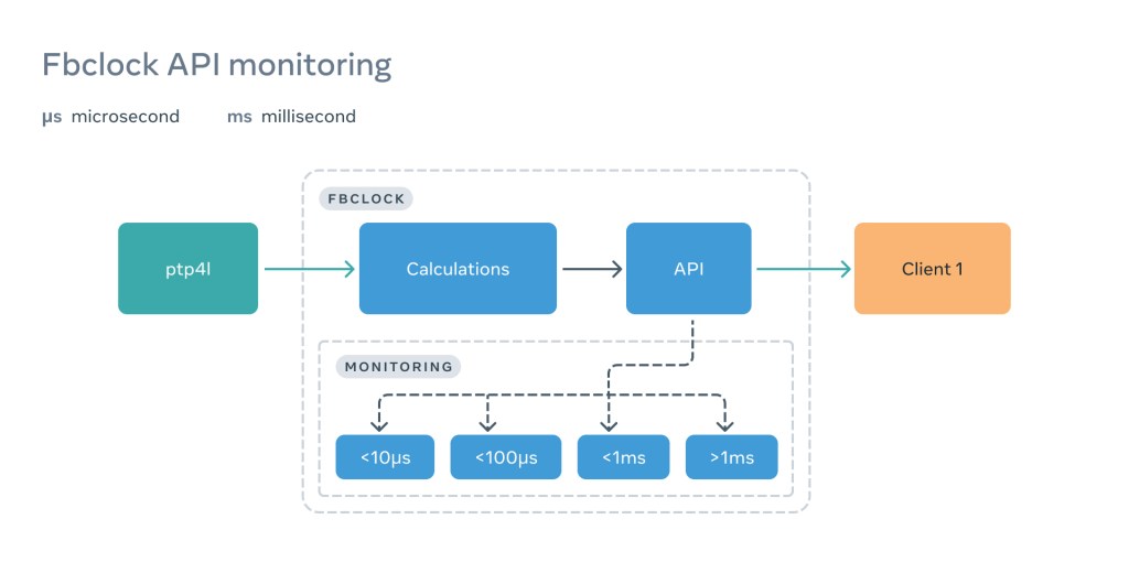
This allows us to clearly see when the client experiences an issue — and often before the client even notices it.
Linearizability checks
PTP protocol (and ptp4l in particular) don’t have a quorum selection process (unlike NTP and chrony). This means the client picks and trusts the Time Server based on the information provided via Announce messages. This is true even if the Time Server itself is wrong.
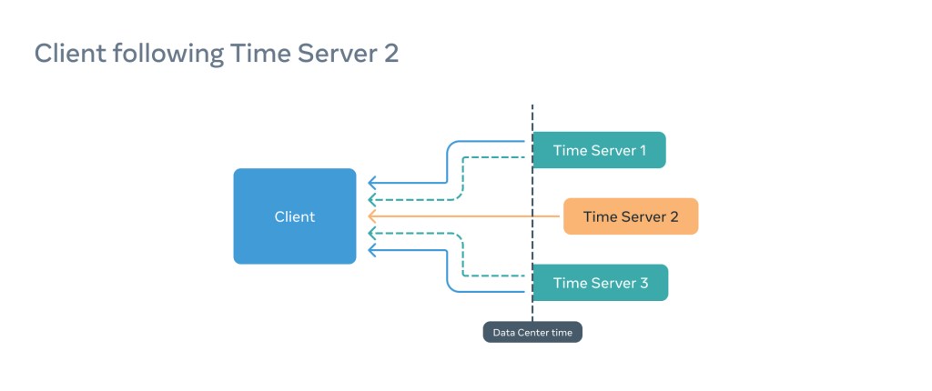
For such situations, we have implemented a last line of defense called a linearizability check.
Imagine a situation in which a client is configured to use three time servers and the client is subscribed to a faulty Time Server (e.g., Time Server 2):
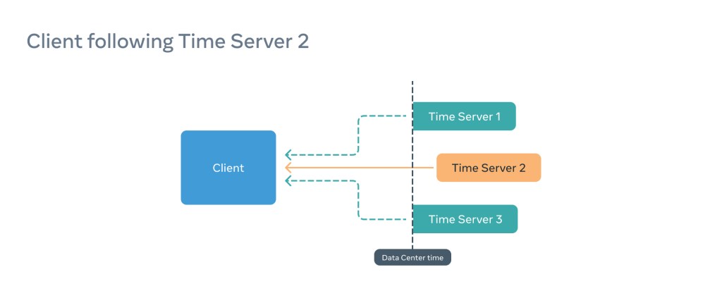
In this situation, the PTP client will think everything is fine, but the information it provides to the application consuming time will be incorrect, as the Window of Uncertainty will be shifted and therefore inaccurate.
To combat this, in parallel, the fbclock establishes communication with the remaining time servers and compares the results. If the majority of the offsets are high, this means the server our client follows is the outlier and the client is not linearizable, even if synchronization between Time Server 2 and the client is perfect.
PTP is for today and the future
We believe PTP will become the standard for keeping time in computer networks in the coming decades. That’s why we’re deploying it on an unprecedented scale. We’ve had to take a critical look at our entire infrastructure stack — from the GNSS antenna down to the client API — and in many cases we’ve even rebuilt things from scratch.
As we continue our rollout of PTP, we hope more vendors who produce networking equipment will take advantage of our work to help bring new equipment that supports PTP to the industry. We’ve open-sourced most of our work, from our source code to our hardware, and we hope the industry will join us in bringing PTP to the world. All this has all been done in the name of boosting the performance and reliability of the existing solutions, but also with an eye toward opening up new products, services, and solutions in the future.
We want to thank everyone involved in this endeavor, from Meta’s internal teams to vendors and manufacturers collaborating with us. Special thanks goes to Andrei Lukovenko, who connected time enthusiasts.
This journey is just one percent finished.


