
People upload hundreds of millions of videos to Facebook every day. Making sure every video is delivered at the best quality — with the highest resolution and as little buffering as possible — means optimizing not only when and how our video codecs compress and decompress videos for viewing, but also which codecs are used for which videos. But the sheer volume of video content on Facebook also means finding ways to do this that are efficient and don’t consume a ton of computing power and resources.
To help with this, we employ a variety of codecs as well as adaptive bitrate streaming (ABR), which improves the viewing experience and reduces buffering by choosing the best quality based on a viewer’s network bandwidth. But while more advanced codecs like VP9 provide better compression performance over older codecs, like H264, they also consume more computing power. From a pure computing perspective, applying the most advanced codecs to every video uploaded to Facebook would be prohibitively inefficient. Which means there needs to be a way to prioritize which videos need to be encoded using more advanced codecs.
Today, Facebook deals with its high demand for encoding high-quality video content by combining a benefit-cost model with a machine learning (ML) model that lets us prioritize advanced encoding for highly watched videos. By predicting which videos will be highly watched and encoding them first, we can reduce buffering, improve overall visual quality, and allow people on Facebook who may be limited by their data plans to watch more videos.
But this task isn’t as straightforward as allowing content from the most popular uploaders or those with the most friends or followers to jump to the front of the line. There are several factors that have to be taken into consideration so that we can provide the best video experience for people on Facebook while also ensuring that content creators still have their content encoded fairly on the platform.
How we used to encode video on Facebook
Traditionally, once a video is uploaded to Facebook, the process to enable ABR kicks in and the original video is quickly re-encoded into multiple resolutions (e.g., 360p, 480p, 720p, 1080p). Once the encodings are made, Facebook’s video encoding system tries to further improve the viewing experience by using more advanced codecs, such as VP9, or more expensive “recipes” (a video industry term for fine-tuning transcoding parameters), such as H264 very slow profile, to compress the video file as much as possible. Different transcoding technologies (using different codec types or codec parameters) have different trade-offs between compression efficiency, visual quality, and how much computing power is needed.
The question of how to order jobs in a way that maximizes the overall experience for everyone has already been top of mind. Facebook has a specialized encoding compute pool and dispatcher. It accepts encoding job requests that have a priority value attached to them and puts them into a priority queue where higher-priority encoding tasks are processed first. The video encoding system’s job is then to assign the right priority to each task. It did so by following a list of simple, hard-coded rules. Encoding tasks could be assigned a priority based on a number of factors, including whether a video is a licensed music video, whether the video is for a product, and how many friends or followers the video’s owner has.
But there were disadvantages to this approach. As new video codecs became available, it meant expanding the number of rules that needed to be maintained and tweaked. Since different codecs and recipes have different computing requirements, visual quality, and compression performance trade-offs, it is impossible to fully optimize the end user experience by a coarse-grained set of rules.
And, perhaps most important, Facebook’s video consumption pattern is extremely skewed, meaning Facebook videos are uploaded by people and pages that have a wide spectrum in terms of their number of friends or followers. Compare the Facebook page of a big company like Disney with that of a vlogger that might have 200 followers. The vlogger can upload their video at the same time, but Disney’s video is likely to get more watch time. However, any video can go viral even if the uploader has a small following. The challenge is to support content creators of all sizes, not just those with the largest audiences, while also acknowledging the reality that having a large audience also likely means more views and longer watch times.
Enter the Benefit-Cost model
The new model still uses a set of quick initial H264 ABR encodings to ensure that all uploaded videos are encoded at good quality as soon as possible. What’s changed, however, is how we calculate the priority of encoding jobs after a video is published.
The Benefit-Cost model grew out of a few fundamental observations:
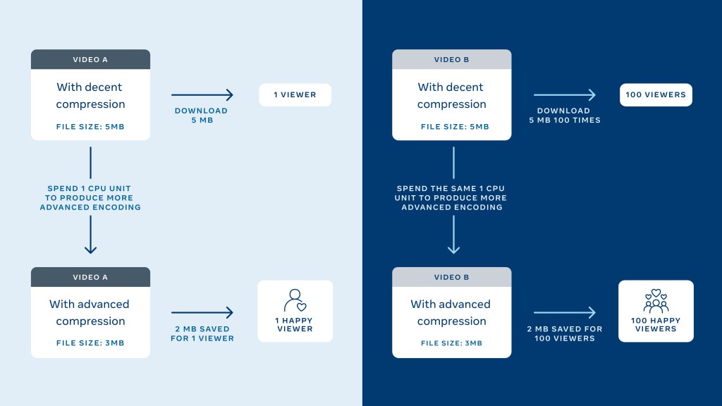
- A video consumes computing resources only the first time it is encoded. Once it has been encoded, the stored encoding can be delivered as many times as requested without requiring additional compute resources.
- A relatively small percentage (roughly one-third) of all videos on Facebook generate the majority of overall watch time.
- Facebook’s data centers have limited amounts of energy to power compute resources.
- We get the most bang for our buck, so to speak, in terms of maximizing everyone’s video experience within the available power constraints, by applying more compute-intensive “recipes” and advanced codecs to videos that are watched the most.
Based on these observations, we came up with following definitions for benefit, cost, and priority:
- Benefit = (relative compression efficiency of the encoding family at fixed quality) * (effective predicted watch time)
- Cost = normalized compute cost of the missing encodings in the family
- Priority = Benefit/Cost
Relative compression efficiency of the encoding family at fixed quality: We measure benefit in terms of the encoding family’s compression efficiency. “Encoding family” refers to the set of encoding files that can be delivered together. For example, H264 360p, 480p, 720p, and 1080p encoding lanes make up one family, and VP9 360p, 480p, 720p, and 1080p make up another family. One challenge here is comparing compression efficiency between different families at the same visual quality.
To understand this, you first have to understand a metric we’ve developed called Minutes of Video at High Quality per GB datapack (MVHQ). MVHQ links compression efficiency directly to a question people wonder about their internet allowance: Given 1 GB of data, how many minutes of high-quality video can we stream?
Mathematically, MVHQ can be understood as:

For example, let’s say we have a video where the MVHQ using H264 fast preset encoding is 153 minutes, 170 minutes using H264 slow preset encoding, and 200 minutes using VP9. This means delivering the video using VP9 could extend watch time using 1 GB data by 47 minutes (200-153) at a high visual quality threshold compared to H264 fast preset. When calculating the benefit value of this particular video, we use H264 fast as the baseline. We assign 1.0 to H264 fast, 1.1 (170/153) to H264 slow, and 1.3 (200/153) to VP9.
The actual MVHQ can be calculated only once an encoding is produced, but we need the value before encodings are available, so we use historical data to estimate the MVHQ for each of the encoding families of a given video.
Effective predicted watch time: As described further in the section below, we have a sophisticated ML model that predicts how long a video is going to be watched in the near future across all of its audience. Once we have the predicted watch time at the video level, we estimate how effectively an encoded family can be applied to a video. This is to account for the fact that not all people on Facebook have the latest devices, which can play newer codecs.
For example, about 20 percent of video consumption happens on devices that cannot play videos encoded with VP9. So if the predicted watch time for a video is 100 hours the effective predicted watch time using the widely adopted H264 codec is 100 hours while effective predicted watch time of VP9 encodings is 80 hours.
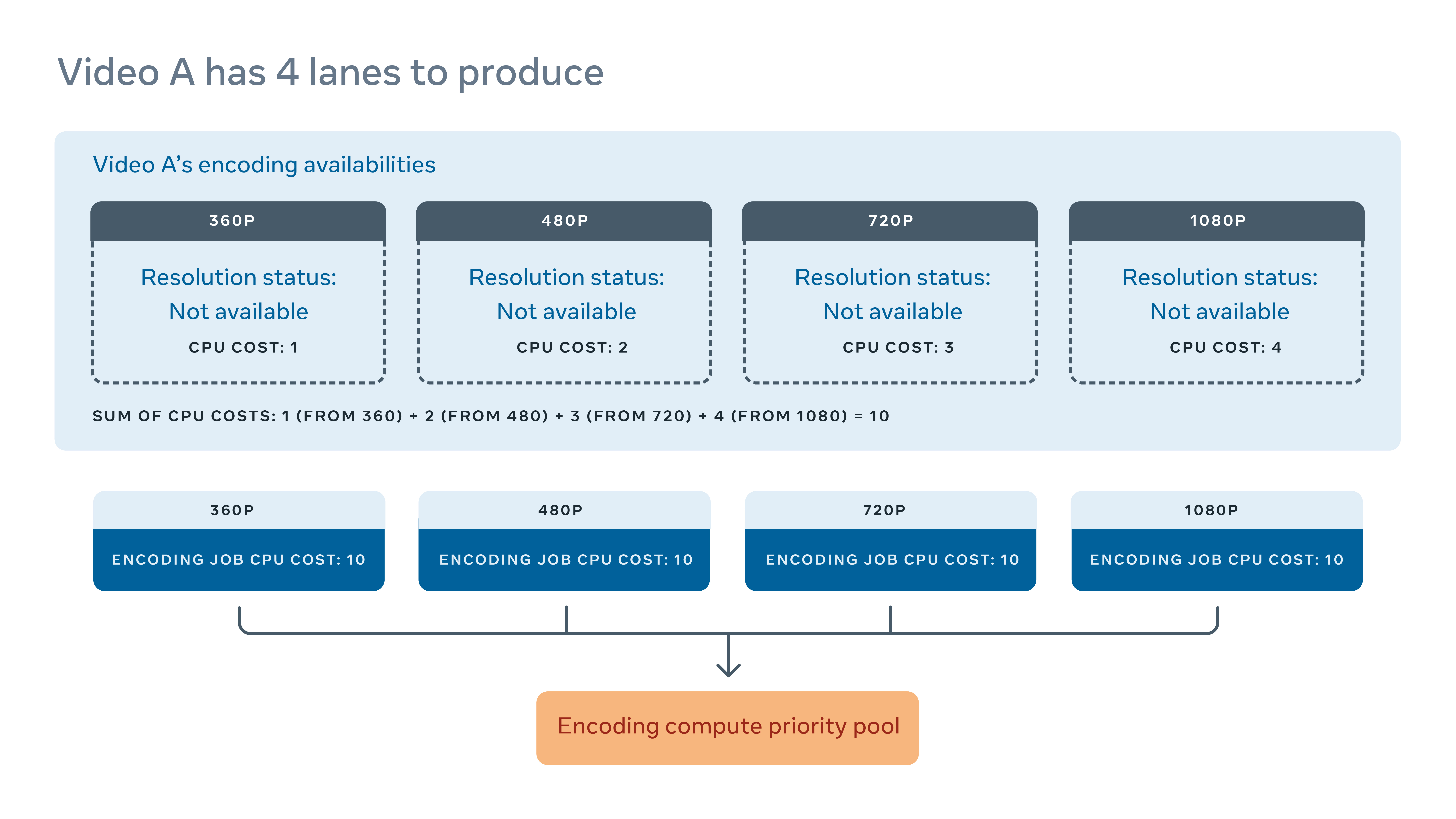
Normalized compute cost of the missing encodings in the family: This is the amount of logical computing cycles we need to make the encoding family deliverable. An encoding family requires a minimum set of resolutions to be made available before we can deliver a video. For example, for a particular video, the VP9 family may require at least four resolutions. But some encodings take longer than others, meaning not all of the resolutions for a video can be made available at the same time.
As an example, let’s say Video A is missing all four lanes in the VP9 family. We can sum up the estimated CPU usage of all four lanes and assign the same normalized cost to all four jobs.
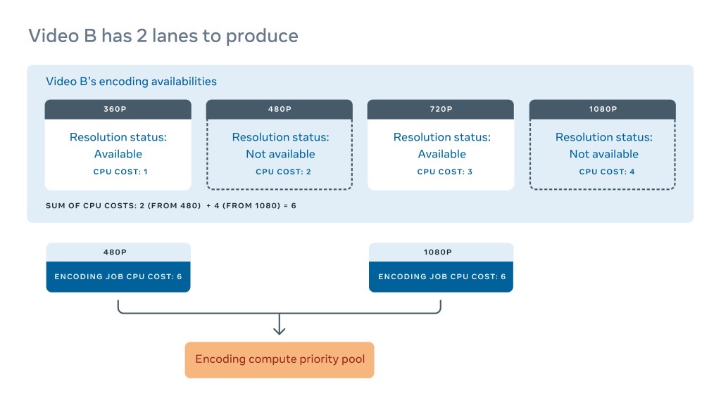
If we are only missing two out of four lanes, as shown in Video B, the compute cost is the sum of producing the remaining two encodings. The same cost is applied to both jobs. Since the priority is benefit divided by cost, this has the effect of a task’s priority becoming more urgent as more lanes become available. Encoding lanes do not provide any value until they are deliverable, so it is important to get to a complete lane as quickly as possible. For example, having one video with all of its VP9 lanes adds more value than 10 videos with incomplete (and therefore, undeliverable) VP9 lanes.
Predicting watch time with ML
With a new benefit-cost model in place to tell us how certain videos should be encoded, the next piece of the puzzle is determining which videos should be prioritized for encoding. That’s where we now utilize ML to predict which videos will be watched the most and thus should be prioritized for advanced encodings.
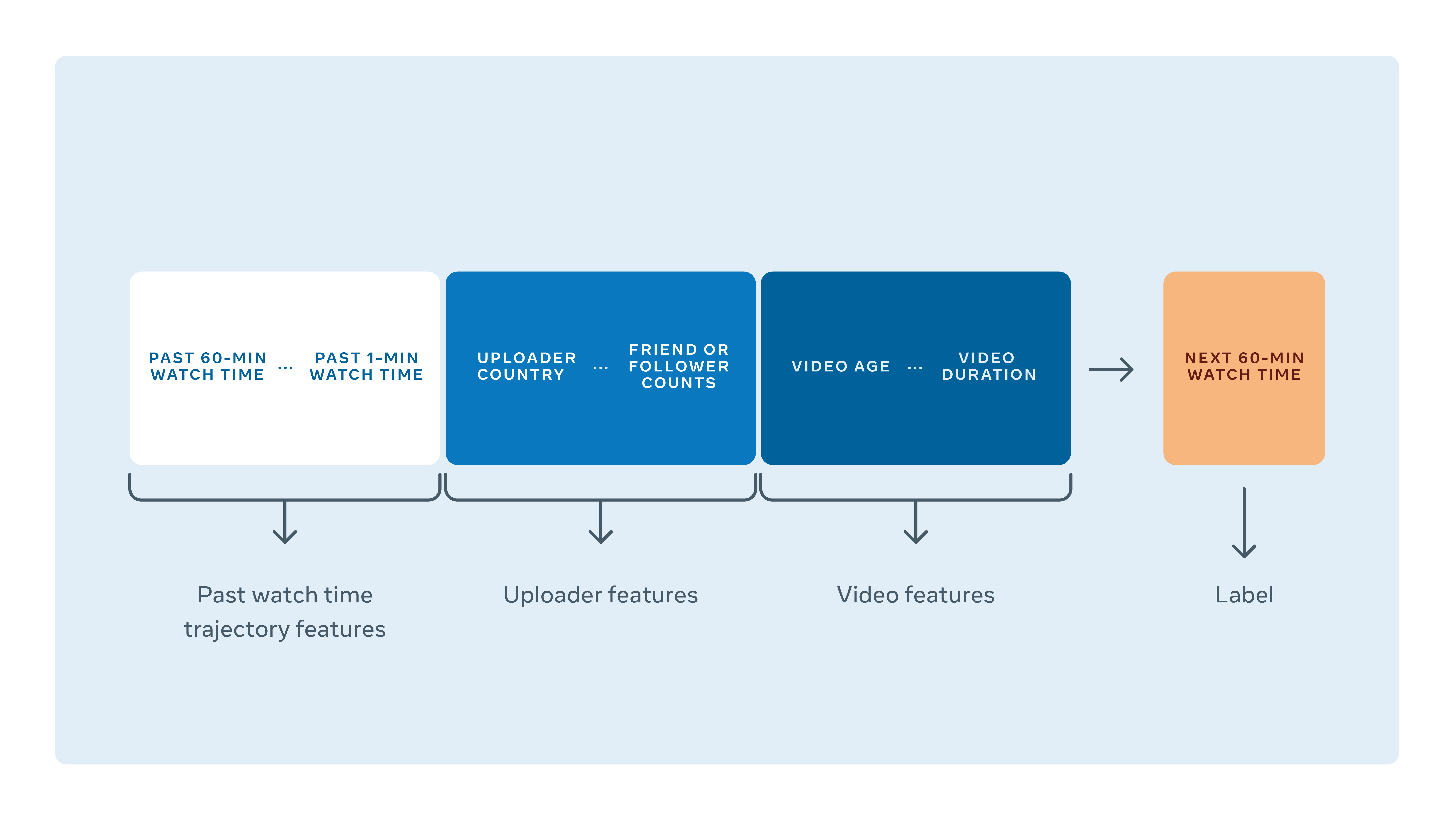
Our model looks at a number of factors to predict how much watch time a video will get within the next hour. It does this by looking at the video uploader’s friend or follower count and the average watch time of their previously uploaded videos, as well as metadata from the video itself including its duration, width, height, privacy status, post type (Live, Stories, Watch, etc.), how old it is, and its past popularity on the platform.
But using all this data to make decisions comes with several built-in challenges:
Watch time has high variance and has a very long-tail skewed nature. Even when we focus on predicting the next hour of watch time, a video’s watch time can range anywhere from zero to over 50,000 hours depending on its content, who uploaded it, and the video’s privacy settings. The model must be able to tell not only whether the video will be popular, but also how popular.
The best indicator of next-hour watch time is its previous watch time trajectory. Video popularity is generally very volatile by nature. Different videos uploaded by the same content creator can sometimes have vastly different watch times depending on how the community reacts to the content. After experimenting with multiple features, we found that past watch time trajectory is the best predictor of future watch time. This poses two technical challenges in terms of designing the model architecture and balancing the training data:
- Newly uploaded videos don’t have a watch time trajectory. The longer a video stays on Facebook, the more we can learn from its past watch time. This means that the most predictive features won’t apply to new videos. We want our model to perform reasonably well with missing data because the earlier the system can identify videos that will become popular on the platform, the more opportunity there is to deliver higher-quality content.
- Popular videos have a tendency to dominate training data. The patterns of the most popular videos are not necessarily applicable to all videos.
Watch time nature varies by video type. Stories videos are shorter and get a shorter watch time on average than other videos. Live streams get most of their watch time during the stream or a few hours afterward. Meanwhile, videos on demand (VOD) can have a varied lifespan and can rack up watch time long after they’re initially uploaded if people start sharing them later.
Improvements in ML metrics do not necessarily correlate directly to product improvements. Traditional regression loss functions, such as RMSE, MAPE, and Huber Loss, are great for optimizing offline models. But the reduction in modeling error does not always translate directly to product improvement, such as improved user experience, more watch time coverage, or better compute utilization.
Building the ML model for video encoding
To solve these challenges, we decided to train our model by using watch time event data. Each row of our training/evaluation represents a decision point that the system has to make a prediction for.
Since our watch time event data can be skewed or imbalanced in many ways as mentioned, we performed data cleaning, transformation, bucketing, and weighted sampling on the dimensions we care about.
Also, since newly uploaded videos don’t have a watch time trajectory to draw from, we decided to build two models, one for handling upload-time requests and other for view-time requests. The view-time model uses the three sets of features mentioned above. The upload-time model looks at the performance of other videos a content creator has uploaded and substitutes this for past watch time trajectories. Once a video is on Facebook long enough to have some past trajectories available, we switch it to use the view-time model.
During model development, we selected the best launch candidates by looking at both Root Mean Square Error (RMSE) and Mean Absolute Percentage Error (MAPE). We use both metrics because RMSE is sensitive to outliers while MAPE is sensitive to small values. Our watch time label has a high variance, so we use MAPE to evaluate the performance of videos that are popular or moderately popular and RMSE to evaluate less watched videos. We also care about the model’s ability to generalize well across different video types, ages, and popularity. Therefore, our evaluation will always include per-category metric as well.
MAPE and RMSE are good summary metrics for model selection, but they don’t necessarily reflect direct product improvements. Sometimes when two models have a similar RMSE and MAPE, we also translate the evaluation to classification problem to understand the trade-off. For example, if a video receives 1,000 minutes of watch time but Model A predicts 10 minutes, Model A’s MAPE is 99 percent. If Model B predicts 1,990 minutes of watch time, Model B’s MAPE will be the same as Model A’s (i.e., 99 percent), but Model B’s prediction will result in the video more likely having high-quality encoding.
We also evaluate the classifications that videos are given because we want to capture the trade-off between applying advanced encoding too often and missing the opportunity to apply them when there would be a benefit. For example, at a threshold of 10 seconds, we count the number of videos where the actual video watch time is less than 10 seconds and the prediction is also less than 10 seconds, and vice versa, in order to calculate the model’s false positive and false negative rates. We repeat the same calculation for multiple thresholds. This method of evaluation gives us insights into how the model performs on videos of different popularity levels and whether it tends to suggest more encoding jobs than necessary or miss some opportunities.
The impact of the new video encoding model
In addition to improving viewer experience with newly uploaded videos, the new model can identify older videos on Facebook that should have been encoded with more advanced encodings and route more computing resources to them. Doing this has shifted a large portion of watch time to advanced encodings, resulting in less buffering without requiring additional computing resources. The improved compression has also allowed people on Facebook with limited data plans, such as those in emerging markets, to watch more videos at better quality.
What’s more, as we introduce new encoding recipes, we no longer have to spend a lot of time evaluating where in the priority range to assign them. Instead, depending on a recipe’s benefit and cost value, the model automatically assigns a priority that would maximize overall benefit throughput. For example, we could introduce a very compute-intensive recipe that only makes sense to be applied to extremely popular videos and the model can identify such videos. Overall, this makes it easier for us to continue to invest in newer and more advanced codecs to give people on Facebook the best-quality video experience.
Acknowledgements
This work is the collective result of the entire Video Infra team at Facebook. The authors would like to personally thank Shankar Regunathan, Atasay Gokkaya, Volodymyr Kondratenko, Jamie Chen, Cosmin Stejerean, Denise Noyes, Zach Wang, Oytun Eskiyenenturk, Mathieu Henaire, Pankaj Sethi, and David Ronca for all their contributions.


