Building an efficient neural language model over a billion words

This post originally appeared on research.facebook.com.

New tools help researchers train state-of-the-art language models

Neural networks designed for sequence predictions have recently gained renewed interested by achieving state-of-the-art performance across areas such as speech recognition, machine translation or language modeling. However, these models are quite computationally demanding, which in turn can limit their application.

In the area of language modeling, recent advances have been made leveraging massively large models that could only be trained on a large GPU cluster for weeks at a time. While impressive, these processing-intensive practices favor exploring on large computational infrastructures that are typically too expensive for academic environments and impractical in a production setting, limiting the speed of research, reproducibility, and usability of the results.

Recognizing this computational bottleneck, Facebook AI Research (FAIR) designed a novel softmax function approximation tailored for GPUs to efficiently train neural network based language models over very large vocabularies. Our approach, called adaptive softmax (more details in the paper), circumvents the linear dependency on the vocabulary size by exploiting the unbalanced word distribution to form clusters that explicitly minimize the expectation of computational complexity. This approach further reduces the computational cost by leveraging the specificities of modern architectures and matrix-matrix vector operations both at train and test time. This makes it particularly suited for GPUs whereas most previous approaches, such as hierachical softmax, NCE, and importance sampling, have been designed for standard CPUs.

FAIR also developed and is open-sourcing a library called torch-rnnlib that allows researchers to design new recurrent models and test these prototypes on GPUs with minimal effort. It also allows seamless access to fast baselines through the torch.cudnn bindings. Several standard recurrent networks such as RNN, LSTM and GRU are already implemented and we show below how one can design new recurrent networks with this library.

These tools and techniques were then applied together against standard benchmarks, such as EuroParl and One Billion Word, which are complex training environments due to the vocabulary sizes used which prohibited us from fitting both a large model and full softmax on GPU. The results demonstrated that we can process 12,500 words/sec on a single GPU, bringing a large gain in efficiency over standard approximations, decreasing the time from experiment to results, all while achieving an accuracy close to that of the full softmax. This will allow for engineers and researchers across academia and industry to train state-of-the-art models with limited resources in short periods of time.

Building a recurrent model with torch-rnnlib

While they are many ways to define recurrent models, we follow this definition: Recurrent networks model sequences of variables over discrete time. It follows the Markov property, that is its future state only depends on its present state.

The simplest recurrent model is Elman’s recurrent model. At each time step t, it produces an output y[t] given its current input variable x[t] and its past state. More precisely, Elman’s recurrent model is defined by the following set of equations:

• h[t] = f(R * h[t-1] + A * x[t]),
• y[t] = B * h[t]

where h represents the (hidden) internal state of the network and f is the sigmoid function. More sophisticated recurrent models have been proposed since then such as the LSTM, GRU or SCRNN.

A good example of application is language modeling, which we now introduce and will be the focus of the remainder of this post.

What is language modeling?

The goal of language modeling is to learn a probability distribution over a sequence of words from a given dictionary. The joint distribution is defined as a product of conditional distribution of words given their past. More precisely, the probability of a sequence of T words w[1],..., w[T] is given as

P(w[1],..., w[T])) = P(w[T]|w[T-1],..., w[1])...P(w[1]).

This problem is traditionally addressed with non-parametric models based on counting statistics (see Goodman, 2001, for details). More recently, parametric models based on recurrent neural networks have gained popularity for language modeling (for example, Jozefowicz et al., 2016, obtained state-of-the-art performance on the 1B word dataset).

How to build a standard model with Torch-rnnlib

We give three different APIs for constructing a network with recurrent connections:

1. The nn.{RNN, LSTM, GRU} interface can be used to construct recurrent networks with the same number of hidden units across all layers.
   • — ‘Import the library’
   • local rnnlib = require ‘rnnlib’
   • — ‘Construct the LSTM network’
   • local lstm = nn.LSTM{inputsize = 256,
   • hidsize = 512,
   • nlayer = 2,}

2. The rnnlib.recurrentnetwork interface can be used to construct recurrent networks with any shape. Both the previous and this interface take care of hidden state saving for you.
3. • — ‘Import the library’
   • local rnnlib = require ‘rnnlib’
   • — ‘Construct the LSTM network’
   • local lstm = rnnlib.makeRecurrent{
   • cellfn = rnnlib.cell.LSTM,
   • inputsize = 256,
   • hids = {512, 512},}

4. The nn.SequenceTable interface can be used to chain computations as a ‘scan’ would. The nn.RecurrentTable constructor is simply a lightweight wrapper that clones the recurrent module over time for you. However, do take note that this is the lowest-level interface and you will have to call rnnlib.setupRecurrent(model, initializationfunctions) in order to setup the recurrent hidden state behaviour.
5. • local rnnlib = require ‘rnnlib’
   • –[[‘The table of cells is fed to each level of
   • the recurrent network to construct each layer.
   • The table of initialization functions helps
   • with the construction of the hidden inputs.’–]]
   • local cells, initfun = {}, {}
   • cells[1], initfun[1] = rnnlib.cell.LSTM(256, 512)
   • cells[2], initfun[2] = rnnlib.cell.LSTM(512, 512)
   • local lstm = nn.SequenceTable{
   • dim = 1,
   • modules = {
   • nn.RecurrentTable{dim = 2,
   • module = rnnlib.cell.gModule(cells[1])},
   • nn.RecurrentTable{dim = 2,
   • module = rnnlib.cell.gModule(cells[2])},
   • }
   • rnnlib.setupRecurrent(lstm, initfun)

Build your own recurrent model

You can also create your own model by defining a function that acts as the cell as well as an initialization function for the cell’s state. There are pre-defined cells in rnnlib.cell such as LSTMs, RNNs, and GRUs. Here’s how you can build an RNN from scratch:

• local rnncell = function(nin, nhid)
• –[[‘The _make function will later be fed
• into rnnlib.cell.gModule to turn it into an
• nn.Module which can then be fed into an
• nn.SequenceTable or nn.RecurrentTable.
• It performs the cell computation.’–]]
• local _make = function(prevh, input)
• local i2h = nn.Linear(nin, nhid, false)(input)
• local h2h = nn.Linear(nhid, nhid, false)(prevh)
• local nexth = nn.Sigmoid()(nn.CAddTable(){i2h, h2h})
• return nexth, nn.Identity()(nexth)
• end
• –[[ ‘The _init function initializes the
• state stored in the cell depending
• on the batch size (bsz).’–]]
• local _init = function(bsz)
• return torch.Tensor(bsz, nhid):fill(0)
• end
• return _make, _init
• end

Train it on GPU

Since torch-rnnlib adheres to the nn module interface, simply call :cuda() on the model to pull it to GPU. The goal of rnnlib is to allow the user flexibility in creating new cells or using fast baselines. On this end, if you use either the first or second API for constructing recurrent networks in the above section you can easily use cudnn to greatly speed up your network. For the nn.{RNN, LSTM, GRU} interface, simply call the constructor with usecudnn = true:

• nn.LSTM{ inputsize = 256,
• hidsize = 512,
• nlayer = 2,
• usecudnn = true}

For the second API, simply replace rnnlib.makeRecurrent with rnnlib.makeCudnnRecurrent and change the cell function to a cell string that is present in the cudnn API. For example:

• rnnlib.makeCudnnRecurrent{
• cellstring = ‘LSTM’,
• inputsize = 256,
• hids = {512, 512},
• }

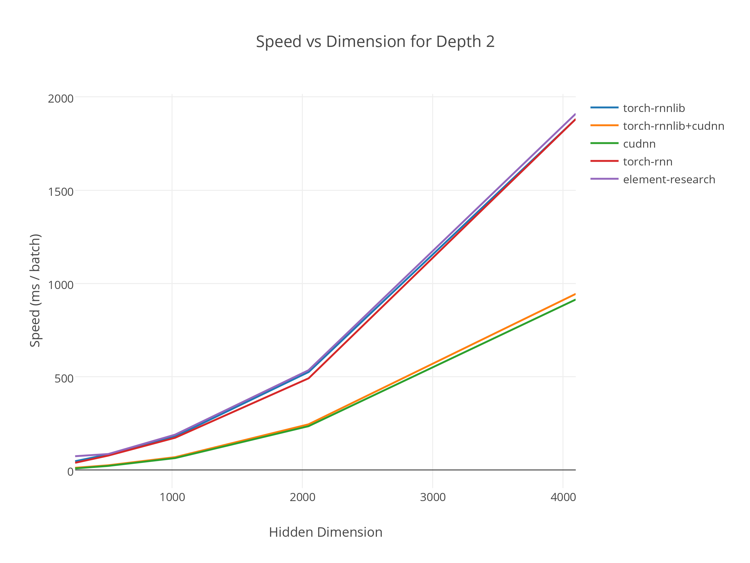
This will generally result in at least a 2x speedup of the recurrent part of the model. Do note that this may not mean a 2x speedup of your whole model, especially if the majority of the computation does not take place in the recurrent portion. For example, if you have a softmax in your model that requires much more computation than the recurrent part, you may only see a 1.3x speedup.

Figure. Comparison of running time as a function of size of the hidden layers between torch-rnnlib and other torch library. We show it with and without using Cudnn. We use an LSTM with 2 layers.

Adaptive-Softmax: a softmax approximation tailored for GPUs

When dealing with large output space (like in language modeling), the classifier can be the computational bottleneck of the model. Many solutions have been proposed in the past (hierarchical softmax, noise contrastive estimation, differentiated softmax) but they are usually designed for standard CPUs and rarely take full advantage of the specificity of GPUs.

We develop a new approximation called the adaptive softmax: A softmax that adapt its computational budget to the distribution of the data. It balances between a good approximation and fast running time by making the most frequent classes faster to access but provides them with more resources. More precisely it learns a k-way hierarchical softmax that takes into account the architecture of the GPUs to assign computation efficiently. This computation allocation can be solved exactly using a simple dynamic programming algorithm. Several tricks have been used to further the computational burden of the classifier: we use shallow trees to avoid sequential computation and we fix a minimum number of classes per cluster to avoid wasting GPUs parallel computation power.

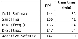
As shown in Table 1, the adaptive softmax almost match the performance of the full softmax while being significantly faster. It also outperforms other approximations on GPUs.

Table 1. Performance on Text8. The lower ppl the better.

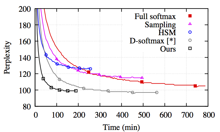
Figure. Convergence of language model with different softmax approximations. It is built on top of an LSTM.

Achieving a perplexity of 45 on the 1-billion word on a single GPU in a couple of days

In terms of technical details, beside the adatpive softmax, we use a relatively standard setting: For our small model we use a LSTM with 1 layer and 2048 units each and for the larger one 2 layers with 2048 neurons each. We train the model using Adagrad (citation needed) and a L2 regularization for the weights. We use a batch size of 128 and we set the back-propagation window size to 20.

Concerning the Adaptative softmax, we use the optimal setting for the distribution of the train set of 1B words, that is 4 clusters with a dimension reduction of x4 over each cluster (see the paper for details).

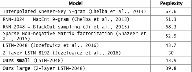
Table 2. Comparison on 1B word in perplexity (lower the better). Note that Jozefowicz et al., uses 32 GPUs for training. We only use 1 GPU.

As shown in table 2, the small model achieve a perplexity of 43.9 within a couple of days. The larger model achieve a perplexity of 39.8 in 6 days. The current state-of-the-art performance is a perplexity of 30.0 (lower the better) and was achieved by Jozefowicz et al., 2016. They achieve this result using 32 GPUs over 3 weeks. They also report a perplexity of 44 achieved with a smaller model, using 18 GPU days to train.

Our small model takes 180 ms/batch and achieves a perplexity of 50 after one epoch (that is ~14hours). Without Cudnn, the small model takes 230 ms/batch which is only 30% slower.

References

1. Chelba, C., Mikolov, T., Schuster, M., Ge, Q., Brants, T., Koehn, P., and Robinson, T. (2013). One billion word benchmark for measuring progress in statistical language modeling. arXiv preprint arXiv:1312.3005.
2. Chen, W., Grangier, D., and Auli, M. (2015). Strategies for Training Large Vocabulary Neural Language Models. arXiv preprint arXiv:1512.04906.
3. Elman, J. L. (1990). Finding structure in time. Cognitive science, 14(2), 179-211.
4. Ji, S., Vishwanathan, S.V.N., Satish, N., Anderson, M.J. and Dubey, P. (2015). BlackOut: Speeding up Recurrent Neural Network Language Models With Very Large Vocabularies. arXiv preprint arXiv:1511.06909.
5. Goodman, J. T. (2001). A bit of progress in language modeling. Computer Speech and Language, 15(4), 403-434.
6. Grave, É., Joulin, A., Cissé, M., Grangier, D., and Jégou, H. (2016). Efficient softmax approximation for GPUs. arXiv preprint arXiv:1609.04309.
7. Jozefowicz, R., Vinyals, O., Schuster, M., Shazeer, N., and Wu, Y. (2016). Exploring the limits of language modeling. arXiv preprint arXiv:1602.02410.
8. Shazeer, N. M., Pelemans, J., and Chelba, C. (2015). Sparse non-negative matrix language modeling for skip-grams.