
- While deploying Precision Time Protocol (PTP) at Meta, we’ve developed a simplified version of the protocol (Simple Precision Time Protocol – SPTP), that can offer the same level of clock synchronization as unicast PTPv2 more reliably and with fewer resources.
- In our own tests, SPTP boasts comparable performance to PTP, but with significant improvements in CPU, memory, and network utilization.
- We’ve made the source code for the SPTP client and server available on GitHub.
We’ve previously spoken in great detail about how Precision Time Protocol is being deployed at Meta, including the protocol itself and Meta’s precision time architecture.
As we deployed PTP into one of our data centers, we were also evaluating and testing alternative PTP clients. In doing so, we soon realized that we could eliminate a lot of complexity in the PTP protocol itself that we experienced during data center deployments while still maintaining complete hardware compatibility with our existing equipment.
This is how the idea of Simple Precision Time Protocol (SPTP) was born.
But before we dive under the hood of SPTP we should explore why the IEEE 1588 G8265.1 and G8275.2 unicast profiles (here, we just call them PTP) weren’t a perfect fit for our data center deployment.
PTP and its limitations
Excessive network communication
A typical IEEE 1588-2019 two-step PTPv2 unicast UDP flow consists of the following exchange:
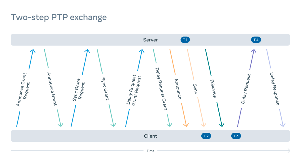
This sequence repeats either in full or in part depending on the negotiation result. The exchange shown is one of many possible combinations. It may involve additional steps such as grant cancellation, grant cancellation acknowledgements, and so on.
The frequency of these messages may vary depending on the implementation and configuration. After completing negotiation, the frequency of some messages can change dynamically.
This design allows for a lot of flexibility, especially for less powerful equipment where resources are limited. In combination with multicast, it allows us to support a relatively large number of clients using either very old or embedded devices. For example, a PTP server can reject the request or confirm a less frequent exchange if the resources are exhausted.
This design, however, leads to excessive network communication, which is particularly visible on a time appliance serving a large number of clients.
State machine
Due to the “subscription” model, both the PTP client and the server have to keep the state in memory. This approach comes with the tradeoffs such as:
- Excessive usage of resources such as memory and CPU.
- Strict capacity limits that mean multicast support is required for large numbers of clients.
- Code complexity.
- Fragile state transitions.
These issues can manifest, for example, in so-called abandoned syncs – situations where the work of a PTP client is interrupted (either forcefully stopped or crashed). Because the PTP server didn’t receive a cancellation signaling message it will keep sending sync and followup packets until the subscription expires (which may take hours). This leads to additional complexity and fragility in the system.
There are additional protocol design side effects such as:
- An almost infinite Denial of Service Attack (DoS) amplification factor.
- Server-driven communication with little control by the client.
- Complete trust in the validity of server timestamps.
- Asynchronous path delay calculations.
In data centers, where communication is typically driven by hundreds of thousands of clients and multicast is not supported, these tradeoffs are very limiting.
SPTP
True to its name, SPTP significantly reduces the number of exchanges between a server and client, allowing for much more efficient network communication.
Exchange
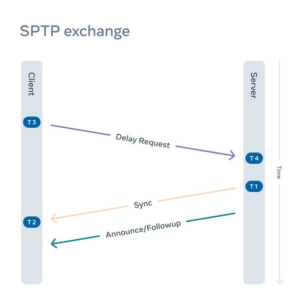
In a typical SPTP exchange:
- The client sends a delay request.
- The server responds with a sync.
- The server sends a followup/announce.
The number of network exchanges is drastically reduced. Instead of 11 different network exchanges as shown on Figure 1 and the requirement for client and server state machines for the duration of the subscription, there are only three packets exchanged and no state needs to be preserved on either side. In the simplified exchange, every packet has an important role:
Delay request
A delay request initiates the SPTP exchange. It’s interpreted by a server not only as a standard delay request containing the correction field (CF1) of the transparent clock, but also as a signal to respond with sync and followup packets. Just like in a two-step PTPv2 exchange, it generates T3 upon departure from the client side and T4 upon arrival on the server side.
To distinguish between a PTPv2 delay request and a SPTP delay request, the PTP profile Specific 1 flag must be set by the client.
Sync
In response to a delay request, a sync packet would be sent containing the T4 generated at an earlier stage. Just like in a regular two-step PTPv2 exchange, a sync packet will generate a T1 upon departure from the server side. While in transit, the correction field of the packet (CF2) is populated by the network equipment.
Followup/announce
Following the sync packet, an announce packet is immediately sent containing T1 generated at a previous stage. In addition, the correction filed from the Delay Request field is populated by the CF1 value collected at an earlier stage.
The announce packet also contains typical PTPv2 information such as clock class, clock accuracy, and so on. On the client side, the arrival of the packet generates the T2 timestamp.
After a successful SPTP exchange, default two-step PTPv2 formulas for mean path delay and clock offset must be applied:
mean_path_delay = ((T4 – T3) + (T2-T1) – CF1 -CF2)/2
clock_offset = T2 – T1 – mean_path_delay
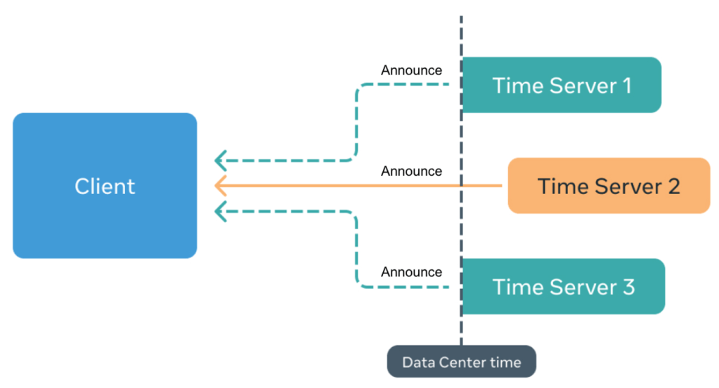
After every exchange the client has access to the announce message attributes such as time source, clock quality, etc., as well as the path delay and a calculated clock offset after every exchange with every server. And, because the exchange is client-driven, the offsets could be calculated at the exact same time. This avoids a situation where a client is following a faulty server and has no chance of detecting it.
Reliability
We can also provide stronger reliability guarantees by using multi-clock reliance.
In our implementation for precision time synchronization, we provide time as well as a window of uncertainty (WOU) to the consumer application via the fbclock API. As we described in a previous blog post on how PTP is being deployed at Meta the WOU is based on the observation of time sync errors for the minimum duration to have stationarity of the state of the system.
In addition, we’ve established a method based on a collection of clocks that each client can access for timing information that we call a clock ensemble. The clock ensemble operates in two modes, steady state and transient; where steady state is during normal operation and transient is in the case of holdover.
However, with a pool of N clocks, C, forming the clock ensemble, the question becomes which clocks to select for determining robustness and accurate timing information. Clocks that are not accurate are rejected (C_reject) and, thus, our ensemble size falls to N = C_total – C_reject. We employ two stages, one that is based on each individual clock, and the second that acts on the collection of valid clocks in the ensemble.
The first stage observes the previous measurements of each individual clock, where the main criteria is to reject outliers in the previous states of the clock. Once this criterion threshold is exceeded, the entire clock is rejected from the valid clock ensemble pool. This is based off Chauvenet’s criterion, where the criterion is a probability band that is centered on the mean of the clock outputs (assuming a normal distribution during steady state). Based on the stationarity tests, we use a sample size of 400 previous clock outputs and calculate a maximum allowable deviation.
For example:
, where
is the current clock output,
is the clock sample mean, and
is the clock set standard deviation.
We find the probability that the current clock output is in disagreement with the previous 400 samples:
Based on a window size of 400 previous samples, the maximum allowed deviation is:
Now, the clock outputs are tested against this value. If they exceed the they are rejected, an alert is raised, and a threshold counter is incremented. Once the rejection threshold is reached for an individual clock, this clock is entirely rejected.
Now, we enter the second stage of verifying the clock ensemble composed of the valid clocks. The second stage forms a weighted average of the non-rejected clocks in the valid clock ensemble, where each clock in the ensemble is reported as its sample size, mean, and variance. The average of the clocks’ means is the weighted average, where the weights are inversely proportional to the mean absolute deviations reported by each clock after applying Chauvenet’s criterion.
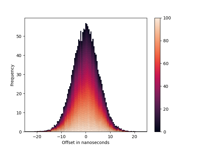
Now we can report the mean and variance of the clock ensemble, ensuring the clocks contained therewith are valid and not providing erroneous values. The confidence interval is scaled with the number of good clocks in the ensemble, where the higher the number of valid clocks out of the total clocks provides greater reliability.
For a number of hosts, we show that the distribution of clocks falls within the following heatmap:
We calculate the variance, , of each individual clock’s observations, then we calculate a weighted mean,
, taking into consideration the reciprocal of each clock’s variance as the weight.
Due to independence of clocks, the variance of the weighted sum, , is:
In summary, we collect samples from a number of clock sources that form our clock ensemble. The overall precision and reliability of the provided data by SPTP is a function of the number of reliable and in distribution clocks forming the clock ensemble.
A future post will focus on this specifically.
SPTP’s performance
Let’s explore performance of the SPTP versus PTP.
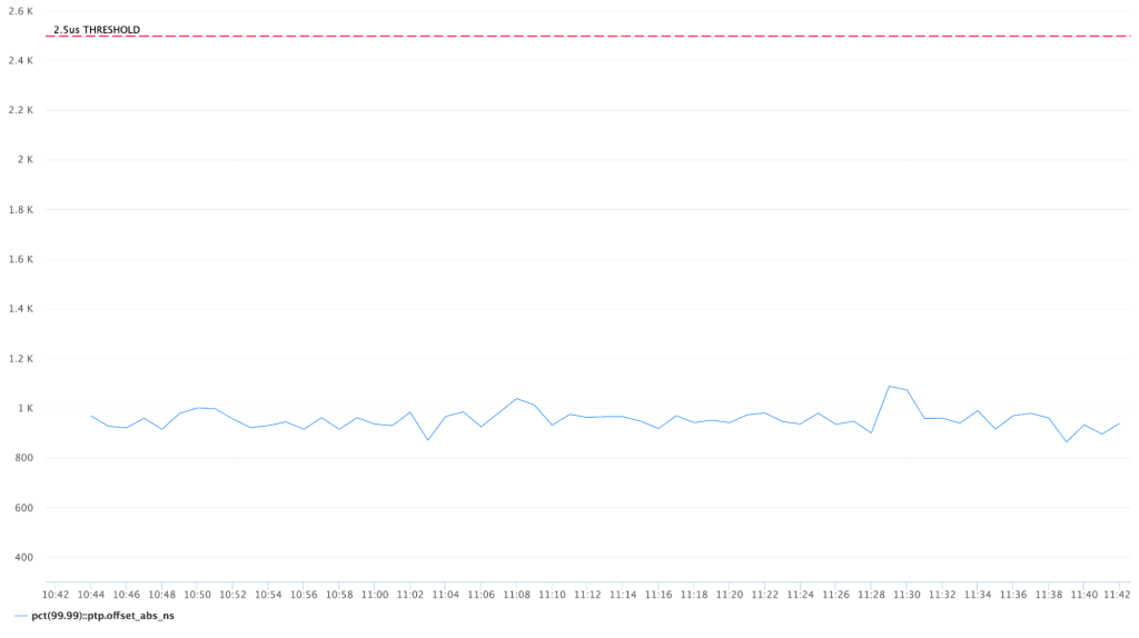
Initial deployments to a single client confirmed no regression in the precision of the synchronization:
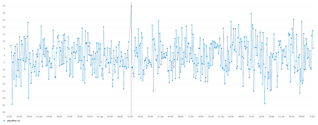
Repeating the same measurement after migration to SPTP produces a very similar result, only marginally different due to a statistical error:
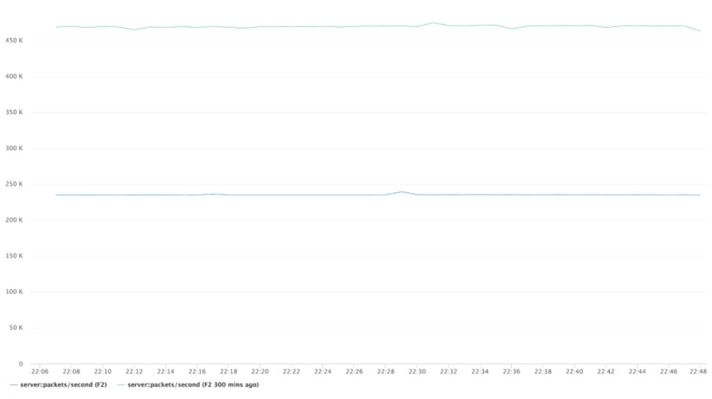
With large-scale deployment of our implementations, we can confirm resource utilization improvements.
We noticed that due to the difference in multi-server support, the performance gains vary significantly depending on the number of tracked time servers.
For example, with just a single time appliance serving the entire network there are significant improvements across the board. Most notably over 40 percent CPU, 70 percent memory, and 50 percent network utilization improvements:
The next steps for SPTP at Meta
Since SPTP can offer the exact same level of synchronization with a lot fewer resources consumed, we think it’s a reasonable alternative to the existing unicast PTP profiles.
In a large-scale data center deployment, it can help to combat frequently changing network paths and create savings in terms of network traffic, memory usage, and number of CPU cycles.
It will also eliminate a lot of complexity inherited from multicast PTP profiles, which is not necessarily useful in the trusted networks of the modern data centers.
It should be noted that SPTP may not be suitable for systems that still require subscription and authentication. But this could be solved by using PTP TLVs (type-length-value).
Additionally, by removing the need for subscriptions, it’s possible to observe multiple clocks – which allows us to provide higher reliability by comparing the time sync from multiple sources at the end node.
SPTP can offer significantly simpler, faster, and more reliable synchronization. Similar to G.8265.1 and G.8275.2 it provides excellent synchronization quality using a different set of parameters. Simplification comes with certain tradeoffs, such as missing signaling messages, that users need to be aware of and decide which profile is the best for them.
Having it standardized and assigned a unicast profile identifier will encourage wider support, adoption, and popularization of PTP as a default precise time synchronization protocol.
The source code for the SPTP client and the server can be accessed on our GitHub page.
Acknowledgements
We would like to thank Alexander Bulimov, Vadim Fedorenko, and Mike Lambeta for their help implementing the code and the math for this article.


")