
The growth of data on the web has made it harder to employ many machine learning algorithms on the full data sets. For personalization problems in particular, where data sampling is often not an option, innovating on distributed algorithm design is necessary to allow us to scale to these constantly growing data sets.
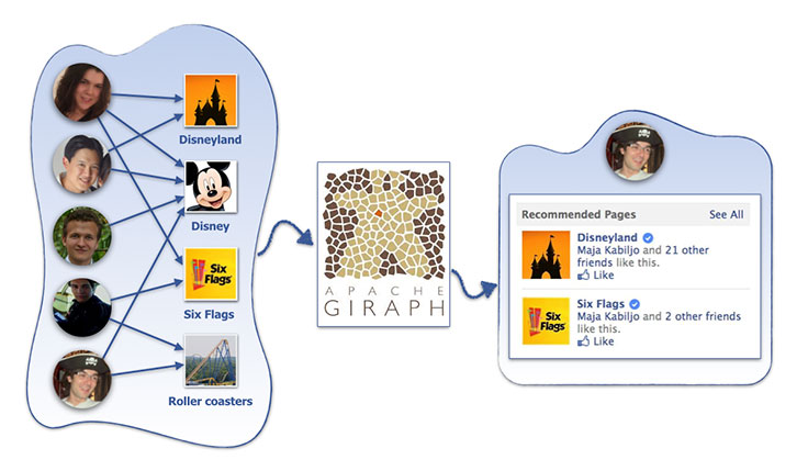
Collaborative filtering (CF) is one of the important areas where this applies. CF is a recommender systems technique that helps people discover items that are most relevant to them. At Facebook, this might include pages, groups, events, games, and more. CF is based on the idea that the best recommendations come from people who have similar tastes. In other words, it uses historical item ratings of like-minded people to predict how someone would rate an item.
CF and Facebook scale
Facebook’s average data set for CF has 100 billion ratings, more than a billion users, and millions of items. In comparison, the well-known Netflix Prize recommender competition featured a large-scale industrial data set with 100 million ratings, 480,000 users, and 17,770 movies (items). There has been more development in the field since then, but still, the largest numbers we’ve read about are at least two orders of magnitude smaller than what we’re dealing with.
A challenge we faced is to design a distributed algorithm that is going to scale to these massive data sets, and how to overcome issues that arose because of certain properties of our data (like skewed item degree distribution, or implicit engagement signals instead of ratings).
As we’ll discuss below, approaches used in existing solutions would not efficiently handle our data sizes. Simply put, we needed a new solution. We’ve written before about Apache Giraph, a powerful platform for distributed iterative and graph processing, and the work we put into making it scale to our needs. We’ve also written about one of the applications we developed on top of it about graph partitioning. Giraph works extremely well on massive data sets, it is easily extensible, and we have a lot of experience in developing highly performant applications on top of it. Therefore, Giraph was our obvious choice for this problem.
Matrix factorization
A common approach to CF is through matrix factorization, in which we look at the problem as having a set of users and a set of items, and a very sparse matrix that represents known user-to-item ratings. We want to predict missing values in this matrix. In order to do this, we represent each user and each item as a vector of latent features, such that dot products of these vectors closely match known user-to-item ratings. The expectation is that unknown user-to-item ratings can be approximated by dot products of corresponding feature vectors, as well. The simplest form of objective function, which we want to minimize, is:
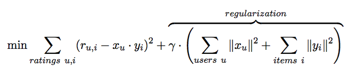
Here, r are known user-to-item ratings, and x and y are the user and item feature vectors that we are trying to find. As there are many free parameters, we need the regularization part to prevent overfitting and numerical problems, with gamma being the regularization factor.
It is not currently feasible to find the optimal solution of the above formula in a reasonable time, but there are iterative approaches that start from random feature vectors and gradually improve the solution. After some number of iterations, changes in feature vectors become very small, and convergence is reached. There are two commonly used iterative approaches.
Stochastic gradient descent optimization
Stochastic gradient descent (SGD) optimization was successfully practiced in many other problems. The algorithm loops through all ratings in the training data in a random order, and for each known rating r, it makes a prediction r* (based on the dot product of vectors x and y) and computes prediction error e. Then we modify x and y by moving them in the opposite direction of the gradient, yielding certain update formulas for each of the features of x and y.
Alternating least square
Alternating least square (ALS) is another method used with nonlinear regression models, when there are two dependent variables (in our case, vectors x and y). The algorithm fixes one of the parameters (user vectors x), while optimally solving for the other (item vectors y) by minimizing the quadratic form. The algorithm alternates between fixing user vectors and updating item vectors, and fixing item vectors and updating user vectors, until the convergence criteria are satisfied.
Standard approach and problems
In order to efficiently solve the above formula in a distributed way, we first looked at how systems that are similar in design to Giraph do it (using message passing instead of map/reduce). The standard approach corresponds to having both users and items as vertices of a graph, with edges representing known ratings. An iteration of SGD/ALS would then send user and/or item feature vectors across all the edges of the graph and do local updates.
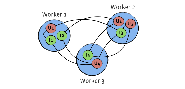
There are a few problems with this solution:
- Huge amount of network traffic: This is the main bottleneck of all distributed matrix factorization algorithms. Since we send a feature vector across each edge of the graph, the amount of data sent over the wire in one iteration is proportional to #Ratings * #Features (here and later in the text we use # as notation for ‘number of’). For 100 billion ratings and 100 double features, this results in 80 TB of network traffic per iteration. Here we assumed that users and items are distributed randomly, and we are ignoring the fact that some of the ratings can live on the same worker (on average, this should be multiplied by the factor 1 – (1 / #Workers)). Note that smart partitioning can’t reduce network traffic by a lot because of the items that have large degrees, and that would not solve our problem.
- Some items in our data sets are very popular, so item degree distribution is highly skewed: This can cause memory problems — every item is receiving degree * #Features amount of data. For example, if an item has 100 million known ratings and 100 double features are used, this item alone would receive 80 GB of data. Large-degree items also cause processing bottlenecks (as every vertex is atomically processed), and everyone will wait for a few largest-degree items to be finished.
- This does not implement SGD exactly in the original formulation: Every vertex is working with feature vectors that it received in the beginning of the iteration, instead of the latest version of them. For example, say item A has ratings for users B and C. In a sequential solution, we’d update A and B first, getting A’ and B’, and then update A’ and C. With this solution, both B and C will be updated with A, the feature vector for the item from the beginning of the iteration. (This is practiced with some lock-free parallel execution algorithms and can slow down the convergence.)
Our solution — rotational hybrid approach
The main problem is sending all updates within each iteration, so we needed a new technique of combining these updates and sending less data. First we tried to leverage aggregators and use them to distribute item data, but none of the formulas we tried for combining partial updates on the item feature vectors worked well.
We finally came up with an approach that required us to extend Giraph framework with worker-to-worker messaging. Users are still presented as the vertices of the graph, but items are partitioned in #Workers disjoint parts, with each of these parts stored in global data of one of the workers. We put all workers in a circle, and rotate the items in clockwise direction after each superstep, by sending worker-to-worker messages containing items from each worker to the next worker in the line.
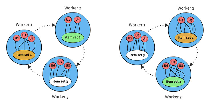
This way, in each superstep, we process part of the worker’s user ratings for the items that are currently on the worker, and therefore process all ratings after #Workers supersteps. Let’s analyze the issues the previous solutions had:
- Amount of network traffic: For SGD, the amount of data sent over the wire in one iteration is proportional to #Items * #Features * #Workers, and it doesn’t depend on the number of known ratings anymore. For 10 million items, 100 double features, and 50 workers, this brings a total of 400 GB, which is 20x smaller than in the standard approach. Therefore, for #Workers <= #Ratings / #Items rotational approach performs much better, i.e., if the number of workers is less than the average item degree. In all data sets that we are using, the items with small degree are ignored from consideration, as those do not represent good recommendations and can be just noise, so average item degree is large. We’ll talk below more about ALS.
- Skewed item degrees: This is no longer a problem — user vertices are the only ones doing processing, and items never hold information about their user ratings.
- Computation of SGD: This is equal as in a sequential solution, because there is only one version of a feature vector at any point of time, instead of having copies of them sent to many workers and doing updates based on that.
The computation with ALS is trickier than with SGD, because in order to update a user/item, we need all its item/user feature vectors. The way updates in ALS actually go is that we are solving a matrix equation of type A * X = B, where A is #Features x #Features matrix and B is 1 x #Features vector, and A and B are calculated based on user/item feature vectors forming all known ratings for item/user. So when updating items, instead of rotating just their feature vectors, we can rotate A and B, update them during each of #Workers supersteps and calculate new feature vectors in the end. This increases the amount of network traffic to #Items * #Features2 * #Workers. Depending on proportions between all the data dimensions, for some items this is better than the standard approach, and for some it isn’t.
This is why a blend of our rotational approach and the standard approach gives the superior solution. By looking at item with some degree, in the standard approach the amount of network traffic associated with it is degree * #Features, and with our rotational approach, it’s #Workers * #Features2. We’ll still update items in which degree < #Workers * #Features using the standard approach, and we’ll use our rotational approach for all larger-degree items, and therefore significantly improve performance. For example, for 100 double features and 50 workers, the item degree limit for choosing an approach is around 5,000.
To solve the matrix equation A * X = B we need to find the inverse A-1, for which we use open source library JBLAS, which had the most efficient implementation for the matrix inverse.
As SGD and ALS share the same optimization formula, it is also possible to combine these algorithms. ALS is computationally more complex than SGD, and we included an option to do a combination of some number of iterations of SGD, followed by a single iteration of ALS. For some data sets, this was shown to help in the offline metrics (e.g., root mean squared error or mean average rank).
We were experiencing numerical issues with large-degree items. There are several ways of bypassing this problem (ignoring these items or sample them), but we were using regularization based on the item and user degrees. That keeps the values for user and item vectors in a certain numerical range.
Evaluation data and parameters
In order to measure the quality of recommendations, before running an actual A/B test, we can use a sample of the existing data to compute some offline metrics about how different our estimations are from the actual user preferences. Both of the above algorithms have a lot of hyperparameters to tune via cross-validation in order to get the best recommendations, and we provide other options like adding user and item biases.
The input ratings can be split in two data sets (train and test) explicitly. This can be very useful in cases in which testing data is composed of all user actions in the time interval after all training instances. Otherwise, to construct the test data, we randomly selected T=1 items per user, and keep them apart from training.
During the algorithm, for a certain percent of users we rank all unrated items (i.e., items that are not in the training set) and observe where training and testing items are in the ranked list of recommendations. Then we can evaluate the following metrics: mean average rank (the position in the ranked list, averaged over all test items), precision at positions 1/10/100, mean of the average precision across all test items (MAP), etc. Additionally we compute root mean squared error (RMSE), which amplifies the contributions of the absolute errors between the predictions and the true values. To help monitor convergence and quality of results, after each iteration we are printing all these metrics.
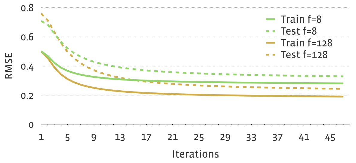
On a sample data set with 35 billion weighted training ratings and 0.2 billion testing ratings, the following figure shows how RMSE reduces on training and testing sets for #Features=8 or #Features=128, where other parameters are fixed.
Item recommendation computation
In order to get the actual recommendations for all users, we need to find items with highest predicted ratings for each user. When dealing with the huge data sets, checking the dot product for each (user, item) pair becomes unfeasible, even if we distribute the problem to more workers. We needed a faster way to find the top K recommendations for each user, or a good approximation of it.
One possible solution is to use a ball tree data structure to hold our item vectors. A ball tree is a binary tree where leafs contain some subset of item vectors, and each inner node defines a ball that surrounds all vectors within its subtree. Using formulas for the upper bound on the dot product for the query vector and any vector within the ball, we can do greedy tree traversal, going first to the more promising branch, and prune subtrees that can’t contain the solution better than what we have already found. This approach showed to be 10-100x faster than looking into each pair, making search for recommendations on our data sets finish in reasonable time. We also added an option to allow for specified error when looking for top recommendations to speed up calculations even more.
Another way the problem can be approximately solved is by clustering items based on the item feature vectors — which reduces the problem to finding top cluster recommendations and then extracting the actual items based on these top clusters. This approach speeds up the computation, while slightly degrading the quality of recommendations based on the experimental results. On the other hand, the items in a cluster are similar, and we can get a diverse set of recommendations by taking a limited number of the items from each cluster. Note that we also have k-means clustering implementation on top of Giraph, and incorporating this step in the calculation was very easy.
Comparison with MLlib
Spark MLlib is a very popular machine-learning library that contains one of the leading open source implementations in this domain. In July 2014, the Databricks team published performance numbers of their ALS implementation on Spark. Experiments were conducted on scaled copies of the Amazon reviews data set, which originally contained 35 million ratings and ran for five iterations.
In the following graph, we compared our rotational hybrid approach (which we implemented in Giraph) with the standard approach (implemented in Spark MLlib, including some additional optimizations, like sending a feature vector at most once to a machine), on the same data set. Due to hardware differences (we had about twice the processing power per machine), in order to make a fair comparison we were looking at total CPU minutes. Rotational hybrid solution was about 10x faster.
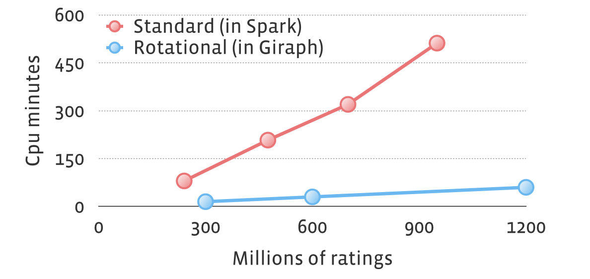
Additionally, the largest data set on which experiments were conducted with standard approach had 3.5 billion ratings. With rotational hybrid approach, we can easily handle more than 100 billion ratings. Note that quality of results is the same for both, and all performance and scalability gains come from different data layout and decreased network traffic.
Facebook use cases and implicit feedback
We used this algorithm for multiple applications at Facebook, e.g. for recommending pages you might like or groups you should join. As already mentioned, our data sets are composed of more than 1 billion users and usually tens of millions of items. There are actually many more pages or groups, but we limit ourselves to items that pass a certain quality threshold — where the simplest version is to have the item degree greater than 100. (Fun side note: On the other side, we have some very large-degree pages — the “Facebook for Every Phone” page is actually liked by almost half of Facebook’s current monthly active users.)
Our first iterations included page likes/group joins as positive signals. The negative signals on Facebook are not as common (negative signals include unliking a page or leaving a group after some time). Also this may not actually mean that a user has negative feedback for that item; instead, he or she might have lost interest in the topic or in receiving updates. In order to get good recommendations, there is a significant need for adding negative items from the unrated pairs in the collection. Previous approaches include randomly picking negative training sample from unrated items (leading to a biased, non-optimal solution) or treating all unknown ratings as negative, which tremendously increases complexity of the algorithm. Here, we implemented adding random negative ratings by taking into account the user and item degrees (adding negative ratings proportional to the user degree based on the item degree distribution), and weighing negative ratings less than positive ones, as we failed to learn a good model with uniform random sampling approach.
On the other hand, we have implicit feedback from users (whether the user is actively viewing the page, liking, or commenting on the posts in the group). We also implemented a well-known ALS-based algorithm for implicit feedback data sets. Instead of trying to model the matrix of ratings directly, this approach treats the data as a combination of binary preferences and confidence values. The ratings are then related to the level of confidence in observed user preferences, rather than explicit ratings given to items.
After running the matrix factorization algorithm, we have another Giraph job of actually computing top recommendations for all users.
The following code just shows how easy it is to use our framework, tune parameters, and plug in different data sets:
CFTrain(
    ratings=CFRatings(table='cf_ratings'),
    feature_vectors=CFVectors(table='cf_feature_vectors'),
    features_size=128,
    iterations=100,
    regularization_factor=0.02,
    num_workers=5,
)
CFRecommend(
    ratings=CFRatings(table='cf_ratings'),
    feature_vectors=CFVectors(table='cf_feature_vectors'),
    recommendations=CFRecommendations(table='cf_recommendations'),
    num_recommendations=50,
    num_workers=10,
)
Furthermore, one can simply implement other objective functions (such as rank optimizations or neighboring models) by extending SGD or ALS computation.
Scalable CF
Recommendation systems are emerging as important tools for predicting user preferences. Our framework for matrix factorization and computing top user recommendations is able to efficiently handle Facebook’s massive data sets with 100 billion ratings. It is easy to use and extend with other approaches.
We are thinking about many improvements and algorithms, including:
- Incorporating the social graph and user connections for providing a better set of recommendations
- Starting from the previous models instead of random initialization, for recurrent learning
- Automatic parameter fitting with cross-validation for optimizing the different metrics for a given data set
- Trying out better partitioning and skipping machines that don’t need certain item data during rotations
We are actively working on recommendations and many other applications on top of Giraph, so stay tuned for more exciting features and development in this field.
Thanks to Dionysios Logothetis, Avery Ching, Sambavi Muthukrishnan and Sergey Edunov from the Giraph team who made this work possible and helped write this story, and Liang Xiong and Bradley Green for early experimentation and all feedback and insights.


